Research Article

Supply Response of Unirrigated Wheat in Khyber Pakhtunkhwa, Pakistan: ARDL Approach

Muhammad Waqas, Shahid Ali*, Syed Attaullah Shah and Ghaffar Ali

Department of Agricultural and Applied Economics, The University of Agriculture, Peshawar, Khyber Pakhtunkhwa, Pakistan.

Received | March 06, 2019; Accepted |June 30, 2019; Published | August 28, 2019

*Correspondence | Shahid Ali, Assistant Professor, Department of Agricultural and Applied Economics, The University of Agriculture, Peshawar, Khyber Pakhtunkhwa, Pakistan; Email: drshahid@aup.edu.pk

Citation | Waqas, M., S. Ali, S.A. Shah and G. Ali. 2019. Supply response of unirrigated wheat in Khyber Pakhtunkhwa, Pakistan: ARDL approach. Sarhad Journal of Agriculture, 35(3): 902-912.

DOI | http://dx.doi.org/10.17582/journal.sja/2019/35.3.902.912

Keywords | Unirrigated wheat, Time series, Supply response, ARDL, Khyber Pakhtunkhwa, Pakistan

Introduction

Agriculture area continues to play a significant position in Pakistan’s economic system. It is far the second largest segment, accounting for over 18.9 percentage of GDP, involves 42.3% of labor force while 62% of the country’s residents exist in rural regions (GoP, 2017). In Pakistan value addition of wheat is 9.1% to agriculture and contributes 1.7% to GDP. Area under wheat crop decreased to 8,734 thousand hectares in 2018 in contrast with previous years of area 8,972 thousand hectares which shows decrease of 2.6 % over the last year. Production of wheat decreased from 26.67 million tons to 25.49 from previous year constitute of decreased in 4.4 % as compared to last years. Per hectare yield of wheat increased due to enhancement in supply of inputs (GoP, 2018).

In world, during 2016, area under wheat harvested was 220.157 million hectares while total wheat production was 749.46 million metric tons (MMT) and having yield of 3405 kg/ha. As far as highest wheat producer of the world in terms of production is concerned, China is on the top of having the production of 131.66 (MMT) followed by India, Russia, America. Canada, France, Ukraine, Pakistan, Germany and Australia. Pakistan is 8th highest wheat producer in the world with the production of 26.0 MMT, on 9.143097 million hectares with 2844.2 kg/ha yield (FAO, 2016).

In Pakistan highest wheat producer province is Punjab followed by Sindh, Khyber Pakhtunkhwa and Baluchistan. Total wheat production in Punjab province was 19526.7 thousand tons on area of 6913.9 thousand hectares. Sindh province was the second largest producer wheat with the production of 3834.6 thousand tons on area 1154.6 thousand hectares. Khyber Pakhtunkhwa was the third producer of producer of wheat with the production of 1400.5 thousand tons on area of 772.3 thousand hectares. In Balochistan 871.3 thousand tons wheat was produced on 382.9 thousand hectares area (GoP, 2016).

For increasing the output of wheat in an area agricultural economics is concerned with one of the most important aspects which need a lot of attention is supply response. It tells about how much the farmers are responsive towards economic incentives (income, profit, rewards etc.). For growth of agriculture response elasticities are very important for policy makers to take decisions about commodities. Differentiation between supply function and supply response is that supply function only tells about the relationship of price and quantity supplied and keeping other things constant. It is a static concept while the supply response conception is dynamic change in prices brings the change in quantity and also discuss supply shifters (Tripathi, 2008).

In literature product level and aggregate level study is done on supply response. The emphasis in product level study is mostly given to the change in product composition or change in planted area in respect of change in the prices of commodities. In aggregate level study the change in entire output of agriculture with respect to change in prices of agriculture in contrast to the prices of industries. Price variations and non-price factors to production like weather change, technology, and input prices are examined in product supply response in order to advance the mechanism of price on micro level which shows either extra tax in sector add to the welfare of economy or the quantity manufactured is significantly increased by price incentives (Ozkan et al., 2011).

Besides own price supply is also influenced by others factors like weather, area, irrigation, price of the substitute, climate, technology and its function are not being undervalued if there is no authentic information about elasticity of supply. So, prediction about short and long run of input on output and designing of agriculture policies are not be achievable (Moula, 2010). Analysis of price elasticities and producer’s response is significant zone in research price mechanism has a very important role in bringing both demand and supply in equilibrium in order to correct the imbalances (Lahiri and Roy, 1985).

In developing countries government mostly favour tax implicitly or explicitly on agriculture sector for the better growth of industries. It is supported by the idea that agriculture sector is static and unresponsive while industry is a dynamic sector. If the supply response is small then taxation on agriculture (changing the internal TOT against agriculture) will produce resources for the other sector in the economy and agriculture growth cannot be upset by the imposition of tax, on the other hand if agriculture supply response is high then taxation on agriculture can slow down the rate of growth of the economy (Chhibber, 1989; McKay et al., 1999).

Pakistan’s population has been growing very rapidly and its population is 210-220 million (GoP, 2017). With the increase in population, demand for wheat is increasing day by day. Most of the area under wheat in Khyber Pakhtunkhwa province is unirrigated. Out of the total area under wheat crop, 429.34 thousand hectares (55.6%) is unirrigated and 343.0 thousand hectares (44.4%) is irrigated (Government of Khyber Pakhtunkhwa, 2017). In the last 30 years, production of unirrigated wheat has been decreased due to overpopulation and the less profitability (Majeed and Shahid, 2009). This fact necessitates efficient utilization of unirrigated land for enhancing wheat production. There is a dire need to gauge the response of farmers of unirrigated areas of province to price and non-price incentives. This will help in framing appropriate policies for unirrigated wheat crop to fill the gap between demand and supply.

For increasing production and income, pricing policy of agriculture has very significant part and supply response is used for understanding this mechanism (Nerlove and Bachman, 1960). Regression of non-stationary time series provide high R2 and significant results but gives spurious/nonsense regression hence results are misleading. Modern approach on the basis of order of integration Pesaran et al. (2001) proposed auto regressive distributed lag model (ARDL) when the order of integration is mixed I (0) and I (1) but not I (2). This study therefore applied ARDL approach to capture response of wheat growers of unirrigated area of Khyber Pakhtunkhwa.

This study applied recent developments in time series analysis. Reliable estimates of supply response of farmer using ARDL approach is important for policy makers. These findings may be useful in formulating wheat policy in unirrigated areas of the country. Farmers may also be benefited from the findings of this study by keeping in view price and non-price variables. Findings of this study are also important for researchers in comparing their results with this study. This study is also an addition to literature as no such study has been conducted on unirrigated wheat in the study area. The main objective of this attempt was to estimate supply response of unirrigated wheat in Khyber Pakhtunkhwa province of Pakistan during 1981-2017.

Materials and Methods

Universe of the study

This study was carried out in Khyber Pakhtunkhwa province situated in the Northern western area of Pakistan having North latitude between 31o15’ and 36o 57 and East longitude is 69o 5’ and 74o 7’. The length between the parallels is 408 miles and its determined breadth between the meridians is 279 miles. On the basis of economy and population it is third largest province. Agriculture is the main occupation in the province and most cash crops are grown in this area. Almost all the districts grow wheat in Khyber Pakhtunkhwa. Most of the area in Khyber Pakhtunkhwa is unirrigated. The total area cultivated under wheat is 772.3 thousand hectares in which unirrigated area is 429.3 thousand hectares and irrigated land is 343.0 thousand hectares having 55.6% and 44.4% share, respectively. As most of the area in Khyber Pakhtunkhwa is un-irrigated, therefore the arid wheat has been taken as the universe of the study.

Data and data sources

Secondary data on unirrigated wheat production, unirrigated area under wheat crop, price of wheat, price of check pea, temperature and rainfall during 1981-2017 were used in this study. Data on unirrigated wheat production (000 tons) and unirrigated area under wheat (000 hectares) were obtained from Development Statistics of Khyber Pakhtunkhwa and Agricultural Statistics of Pakistan. Data on prices of wheat (Rs/100 kg) and chick pea (Rs/100 kg) were taken from Development Statistics of Khyber Pakhtunkhwa and Pakistan Bureau of Statistics. Data regarding maximum and minimum temperature (0C) and rainfall (mm) were taken from Pakistan Metrological Department, Peshawar.

Data analysis

Conceptual framework: Supply response model was first used by Nerlove (1958). This Nerlovian model tells about the price and quantity expectation. The Nerlovian model is dynamic in nature (its previous and lagged values explain the dependent variable. Nerlovian model is auto regressive model due to its lagged values (Leaver, 2004). Change in variable is defined by the partial adjustment model λ, showing a change between the desired level of output and the present level of output (Kennedy, 2008).

λb1 is the short run price elasticity and (1-λ) shows the long run elasticity.

The criticism on Nerlovian model is that it gives misleading results or spurious regression (McKay et al. 1999). Moreover, Nerlovian model gives high R2 and significant value but the results are spurious (Granger and Newbold, 1974). It means if one non-stationary time series is regressed on another non stationary time series; it gives the spurious regression. The identification of spurious regression is that the R-square value will be greater than Durbin Watson statistics. It shows the good fitted model but the results have no meaning. For estimating supply response of farmers, most of the studies e.g., Pinckney (1989), Cummings (1975), Askari and Cummings (1977), Hussain and Sampath (1996), among others, used Nerlovian partial adjustment model (1958) to estimate time series data which is mostly trended over time (non-stationary). In order to tackle this problem, (Box and Jenkins, 1970) introduced a method of differencing but according to (Davidson et al. 1978), it leads us to a loss of long run valuable information. Engle and Granger (1987) introduced a method of cointegration which calculate the long run information. If all the variables are integrated of order 1, ECM (in case of two variables) or VECM (in case of more than two variables) of Johansen and Juselius (1990) is used for cointegration. Most of the studies including Hallam and Zanoli (1992), Townsend and Thirtle (1994), Ajetomobi (2010) and Akanni and Okeowo (2011). Pesaran et al. (2001) proposed auto regressive distributed lag model (ARDL) when the order of integration is mixed I (0) and I (1) but not I (2), ARDL was applied.

Stationary, non-stationary and order of integration

Time series is said to be stationary if it has constant mean, variance and covariance. If thesis statistics are not constant, then the series is non stationary. Variables would be stationary if they don’t exhibit downward or upward trend.

Different tests like DF, ADF, Durbin Watson and Philip-Perron are used to check the problem of stationarity.

Various time series are stationary at different orders known as order of integration. If a time series is stationary at level then this referred to as integrated of order zero i.e., I (0). If a series is stationary at 1st difference, it is said to be integrated of order one written as I (1). If a series is stationary at 2nd difference then this series is referred to as integrated of order two i.e., I (2).

Augmented Dickey Fuller (ADF) test

Dickey fuller test is advanced by two statisticians Dickey and Fuller (Dickey and Fuller, 1981). To check whether the variables are stationary or non-stationary, ADF is widely used, given as:

 

First difference of wt is Δ wt. a is intercept or drift term. n is the maximum length of lagged dependent variable while et is the pure white noise error term. Null hypothesis is H0: Φ = 1 or H0: Φ – 1=0 (non-stationary) while alternative hypothesis is H0: Φ < 1 or H0: Φ - 1<0 (stationary). The Augmented Dickey Fuller test is only applicable when the error term is white noise (no autocorrelation) lag term will be added until Δ wt-i. we don’t have serial correlation in our error term. Additional altering terms are included in right side of equation to make the error term white noise. DF distribution will be invalidated because of serial correlation error and its basis on assumption of white noise et.

Model is selected on the basis of data stationarity. If the data is stationary at level I (0) then simple regression will be is used in which further ECM or VECM will be applied. On the other hand, if some of the data is stationary at level I (0) and some is at 1st difference I (1) then ARDL is used and if the variables are stationary at level I (0),1st difference I (1) and 2nd difference I (2) then Toda and Yommamoto (1995) is used. In current study the ADF and tests suggested ARDL model for estimation of long and short run elasticities.

Lag order selection

Vector auto regression (VAR) was employed for lag order selection. VAR takes in to account Akaike Information Criterion (AIC), Schwarz Information Criterion (SIC), Hannan and Quinn (HQ) and Final Prediction Error (FPE) for selection of lags.

Auto Regressive Distributed lags (ARDL) model

The ARDL was first presented by Pesaran et al. (2001). If some series are stationary at level I(0) and some are stationary at 1st difference I(1) then ARDL is used. ARDL approach has some advantages such as it gives more consistent and reliable results for small data set (Haugh, 2002). It can give more than one long run relationship rather than supposing one cointegrated vector. More options are provided for the selection of correct number of lags for dependent and independent variable. ARDL is applied for estimating both the short and long run coefficients simultaneously. It can give reliable statistical inferences about the long run relationship (Zhai et al., 2017).

Supply response model for unirrigated wheat

Unirrigated wheat’s output is assumed to be a function of its own price (prwh), price of competitive crop (prch), area under unirrigated wheat (auwhT), rainfall during crop season (rainfall) minimum temperature (mint) and maximum temperature (maxt. The estimated equation was first transformed into natural log like Leaver (2004), Mohammad et al. (2007), Muchpondawa (2009) and Shahzad et al. (2018) as follows:

 

Where;

t = 1,2,3,4,5,6,…..37 Time period is from 1981-2017; Inqunwht = Natural log of production; Inprwh = Natural log of price of wheat; Inprcht = Natural log price of price of chick pea; Inaunwh = Natural log area under unirrigated wheat; Inmintt = Natural log of minimum temperature; Inmaxtt = Natural log of maximum temperature; Inrainfall = Natural log of rainfall.

Bound test

For checking the long run relationship between the dependent variable and regressors, the bound test is applied. The model which is used for bound test is given as follows.

 

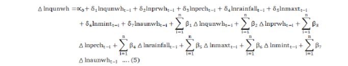
Where;

In is the natural log, ˄ is the difference operator, t-i is used for the lags based on Schwarz and Akaike info criterion, δ and β are the parameters for estimation. For the derivation of optimal lag length for each factor ARDL estimates (p+1)n number of regression. Error correction dynamics are denoted with summation sign. n is the maximum number of lag. β1, β2 β3 β4 β5 β6 and β7 are coefficients showing short run dynamics converging to equilibrium. δ1-δ7 shows the long run relationship among the variables. After estimating the equation mentioned above, F statistics is used for checking the long run relationship among the variables with the null hypothesis of no cointegration.

 

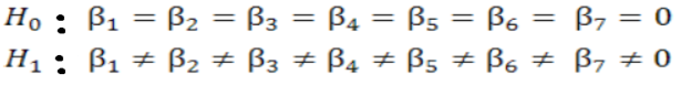
For accepting or rejecting the null hypothesis there are 2 critical bounds, upper and lower bound. If the F-value of bound test is larger than upper bound value at 5% level of significance then null hypothesis is rejected. Moreover, if the F-value is smaller than the lower bound value, then the null hypothesis is accepted. If the F-value is in between the upper and lower bound that would fall in inconclusive zone, showing that there will be no affirmative results and decision cannot be made for the long run relationship. In this study the long run relationship exists therefore long and short run elasticities were estimated.

Long and short run elasticities

Long run elasticities among variables were estimated by using the following equation.

 

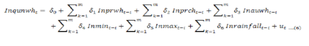
In Equation (6) δi shows long run elasticities of variables. AIC, HQ information criterion are used for the lag selection. To estimate the short run elasticities, the following model was used.

 

Where;

βs are the elasticities of short run, ECT is the error correction term, λ is the coefficient that shows the speed of adjustment towards the long run and its range is in between 0 and -1.

Diagnostics tests

Breusch-Godfrey LM test for serial correlation, Breusch-Pagan-Godfrey test for heteroscedasticity, JB test for normality, Ramsey RESET test for model specification, CUSUM and CUSUMSQ for structural break were used.

Results and Discussion

Descriptive statistics of the variables

Table 1 illustrates descriptive statistics of all variables used in approximation of supply response of unirrigated wheat growers. Production of unirrigated wheat (lnqunwh), price of wheat (lnprwh), price of chickpea (lnprch), area under unirrigated wheat (lnaunwh), minimum temperature (lnmint), maximum temperature (lnmaxt) and rainfall during growing season (lnrainfall) were the major variables of the estimated model. These variables were first transformed into natural log. Mean, standard deviations, minimum, maximum and Jarque-Bera (JB statistics) are presented in table. P-values of JB test showed that the residuals of all the variables were normally distributed except (lnrainfall).

Unit root tests

ADF test: On the basis of graphical inspection, variables were taken with intercept and with trend and intercept. Table 2 presents ADF test results at level and at first difference. The relevant absolute MacKinnon critical values of minimum temperature (lnmint), maximum temperature (lnmaxt) and rainfall (lnrainfall) were greater than the absolute value of ADF test statistics, revealing that the null hypothesis of non-stationarity is rejected for these variables and was concluded that the data is stationary at level I(0). Production of unirrigated wheat (lnqunwh), price of wheat (lnprwh), price of chick pea (lnprch) and area under unirrigated wheat (lnaunwh) were having the MacKinnon critical less than the absolute values of ADF test statistics values at 5% level of significance, showing that the null hypothesis of unit root cannot be rejected. ADF test results indicated that the data has the problem of stationarity at level I(0) but after first difference I(1), the data was stationary.

Table 1: Descriptive statistics of the variables.

Variables	Mean	Std. Dev.	Min	Max	JB Statistics	Prob
lnqunwh	6.153	0.156	5.751	6.445	1.432	0.488
lnprwh	6.583	1.029	4.952	8.179	2.665	0.264
lnprch	7.757	1.099	6.128	9.568	2.795	0.247
lnaunwh	6.138	0.094	5.957	6.305	2.963	0.227
lnmint	1.828	0.132	1.442	2.079	1.731	0.421
lnmaxt	3.014	0.050	2.946	3.122	2.485	0.288
lnrainfall	6.156	0.242	5.327	6.534	14.24	0.001

Source: Authors’ estimates from data, 1981-2017.

Table 2: ADF test.

At Level
Series	ADF statistics	Mackinnon critical value	Prob.	Conclusion
Lnqunwh	-2.82	-2.94	0.060	Non stationary
Lnprwh	-2.43	-3.54	0.350	Non stationary
Lnprch	-3.27	-3.54	0.080	Non stationary
Lnaunwh	-3.09	-3.54	0.123	Non stationary
Lnmint	-3.05	-2.94	0.030	Stationary
Lnmaxt	-4.17	-2.94	0.002	Stationary
lnrainfall	-3.92	-2.94	0.004	Stationary
At First Difference
lnqunwh	-9.10	-2.94	0.000	Stationary
Lnprwh	-5.25	-3.54	0.0007	Stationary
Lnprch	-4.7	-3.54	0.003	Stationary
lnaunwh	-8.9	-3.54	0.000	Stationary

Source: Authors’ estimates from data, 1981-2017.

PP test: Results of Philips-Perron test are presented in Table 3. Phillips Perron test results reinforced the results of ADF test suggesting that Auto Regressive Distributed Lag (ARDL) is appropriate for reliable estimates of long and short run elasticities.

Table 3: PP test.

At Level
Series	PP statistics	Mackinnon critical value	Prob.	Conclusion
lnqunwh	-2.65	-2.94	0.09	Non stationary
lnprwh	-2.56	-3.54	0.29	Non stationary
lnprch	-2.68	-3.54	0.24	Non stationary
lnaunwh	-3.14	-3.54	0.112	Non stationary
lnmint	-5.35	-2.94	0.03	Stationary
lnmaxt	-4.36	-2.94	0.0014	Stationary
lnrainfall	-3.91	-2.94	0.004	Stationary
At First Difference
lnqunwh	-9.16	-2.94	0.0000	Stationary
lnprwh	-5.49	-3.54	0.0004	Stationary
lnprch	-5.87	-3.54	0.0001	Stationary
lnaunwh	-8.9	-3.54	0.000	Stationary

Source: Authors’ estimates from data, 1981-2017.

Lag order selection (VAR): Table 4 presents results of vector auto regression (VAR) results for lag order selection. Final prediction error (FPE), Akaike information (AIC) and Hannan-Quinn (HQ) information criteria proposed the 3 lags in the VAR model. While LR test statistics, Schwarz criteria suggested one lag. Therefore, three lags were used in model for estimation of long and short run elasticities.

Table 4: Lag order selection (VAR).

Lags	Log L	LR	FPE	AIC	SIC	HQ
0	136.867	NA	1.14e-12	-7.639	-7.325	-7.532
1	268.191	200.848*	9.53e-15	-12.48	-9.968*	-11.624
2	322.809	61.0438	1.01e-14	-12.812	-8.098	-11.205
3	414.782	64.9218	2.88e-15*	-15.340*	-8.426	-12.982*

Source: Authors’ estimates from data.

Bound test: Results of bound test are depicted in Table 5. Bound test was used to check the long run relationship. The bound test results verified that the long run relationship between the dependent and explanatory variables does exist as the estimated F value of 11.42 was greater than the upper bound value at all levels of significance.

ARDL results

Long run elasticities: After verifying the long run relationship between the dependent variable and regressors, results of the long run estimated elasticities of ARDL are given in Table 6. Results revealed that price of wheat had a positive and statistically significant relationship with production of unirrigated wheat and its coefficient was 0.447. This means that it is price inelastic and 1% increase in price of wheat increased production by 0.447 percent. Price of chick pea had a negative and significant effect on wheat production and its coefficient was 0.19. This implies that 1% increase in the price of chick pea decreased wheat production by 0.19 percent. It can be inferred that chick pea is competitive crop of wheat in unirrigated areas of Khyber Pakhtunkhwa but its effect on wheat production is inelastic. Results of own price of wheat and price of chick pea price are in conformity with the findings of Fahimifard et al. (2011), Mushtaq and Dawson (2003) and Shahzad et al. (2018). Area under unirrigated wheat had a positive and significant impact on wheat production and its estimated coefficient was 1.10; implies that the effect of area on wheat production is elastic and 1% increase in area under unirrigated wheat increased its production by 1.10%. These results are consistent with the finding of Shahzad et al. (2018) but their estimated coefficient was inelastic (0.868). Minimum temperature had a positive and significant impact on production of wheat and its coefficient was 0.764. This means that 1% increase in minimum temperature increased wheat production by 0.764 percent.

Maximum temperature had negative but insignificant effect on wheat production. Similar results were also obtained by Zhai et al. (2017). Rainfall had a positive and significant effect on production of unirrigated wheat. One percent increase in rainfall increased the production by 0.60 percent and these results are in line with Muchpondawa (2009) and Fahimifard et al. (2011).

Table 5: Bound test.

Test Statistic	Value	K
F-statistic	11.42599	6
	Critical Value Bounds
Significance	I0 Bound	I1 Bound
10%	1.99	2.94
5%	2.27	3.28
1%	2.88	3.99

Source: Authors’ estimates from data, 1981-2017.

Table 6: Long run elasticities.

Variables	Coefficients	Std. Errors	t-ratios	Prob.
Lnprwh	0.447	0.098	4.562**	0.000
Lnprch	-0.194	0.073	-2.656*	0.022
Lnaunwh	1.102	0.404	2.726*	0.019
Lnmint	0.764	0.233	3.284**	0.007
Lnmaxt	-1.209	0.772	-1.566ns	0.145
Lnrainfall	0.608	0.167	3.638**	0.004
Constant	-3.471	5.114	-0.678ns	0.511

Source: Authors’ estimates from data, 1981-2017; Note: ** and * shows level of significance at 1% and 5%, respectively.

Short run elasticities

Table 7 shows short run elasticities of unirrigated wheat production estimated by using ARDL. The lagged value of production of wheat (unirrigated) had positive but insignificant relationship in short run. This result is in correspondence to Ozkan et al. (2011). Price of wheat has negative and statistically significant relationship in short run. One percent increase in price of wheat decreased production of wheat by 0.11% and hence price inelastic. Similar results were obtained by Muchpondawa (2009) and Mushtaq and Dawson (2003). Price of chick pea had negative and significant impact on production of wheat. One percent increase in the prices of chick pea in the short run decreased production of unirrigated wheat by 0.15 percent. One percent increase in rainfall increased production of unirrigated wheat by 0.34 percent. These results are in line with Fahimifard et al. (2011), Muchpondawa (2009). Minimum temperature had positive and significant impact on unirrigated wheat production. One percent increase in minimum temperature increased production by 0.23 percent while maximum temperature had positive but insignificant impact on production of wheat. Similar results were obtained by Riaz (2015). Area unirrigated under wheat had positive relationship with production of wheat as 1% increase in area in short run increased production by 1.79 percent. These results are in line with the results obtained by Shahzad et al. (2018). The value of error correction term (ECT) was estimated -0.97; this means that the process of adjustment is normal and if any disequilibrium occur the whole system will restore to its equilibrium by 97% each year. Similar results were obtained by Leaver (2004) and Muchpondawa (2009).

R-square value was estimated as 0.97, indicating that 94 percent change in the dependent variable was due to the explanatory variables. However, the DW statistics cannot be used for the decision of autocorrelation among the residuals. The DW statistics of 2.20 was greater than the value of R2 (0.97), indicating that the model is effectively reliable. The P-value of the Jarque-Bera was estimated as 0.86, greater than 0.05 which revealed that the data has no problem of normality and the residuals are normally distributed.

Breusch-Godfrey LM test for serial correlation was also conducted. The estimated results determined that there is no serial correlation. The p-value of chi-square was estimated as 0.2 which confirms to accept the null hypothesis of no serial correlation. Breusch-Pagan-Godfrey test of heteroscedasticity confirmed that th e data is homoscedastic as the p-value of chi-square (0.74) suggested to accept the null hypothesis of homoscedastic variance. Ramsey RESET test was conducted for the model adequacy. The p-value of test was 0.11, revealing that the model is adequately specified.

Table 7: Short run elasticities.

Variables	Coefficients	Std. Errors	t-ratios	Prob.
D(lnqunwh)	0.021	0.161	0.135ns	0.895
D(lnprwh)	-0.116	0.043	-2.698*	0.020
D(lnprwh (-1))	-0.079	0.062	-1.288ns	0.223
D(lnprwh (-2))	-0.544	0.057	-9.522**	0.000
D(lnprch)	-0.154	0.031	-4.914**	0.0005
D(lnprch (-1))	0.209	0.030	6.899**	0.000
D(lnaunwh)	1.793	0.168	10.614**	0.000
D(lnaunwh(-1))	-0.431	0.166	-2.588*	0.025
D(lnaunwh(-2))	0.702	0.177	3.955**	0.002
D(lnmint)	0.239	0.081	2.950*	0.013
D(lnmint(-1))	-0.446	0.093	-4.770**	0.000
D(lnmint(-2))	-0.119	0.049	-2.393*	0.035
D(lnmaxt)	-0.054	0.261	-0.208ns	0.839
D(lnmaxt(-1))	1.149	0.260	4.415**	0.001
D(lnrainfall)	0.344	0.037	9.199**	0.000
D(lnrainfall (-1))	-0.194	0.041	-4.772**	0.0006
Cointeq(-1)	-0.978	0.079	-12.230**	0.000
R squared = 0.97; Adjusted R squared = 0.93
Jarque-Bera statistics p value = 0.86
DW statistics = 2.20
Breusch-Godfrey Serial Correlation LM test p-value = 0.20
BPG Heteroscedasticity test p-value = 0.740
Ramsey rest test p-value = 0.11

Source: Authors’ estimates from data, 1981-2017; Note: ** and * shows level of significance at 1% and 5%, respectively.

CUSUM and CUSUMSQ stability tests

These stability tests are based on cumulative sum of recursive residuals and were introduced by Brown et al. (1975). It measures the parameter instability within the range of 5%. When the blue line is in between the two red lines then the estimation is stable. If it goes outside then it is unstable and have structural break. Figure 1 shows that estimation is stable. The implementation of CUSUMSQ test is on squares of residuals. Figure 2 shows that residuals’ variances are within the limits. So the second test of stability is also approved and suggesting that model is reliable.

Conclusions and Recommendations

This study estimated and examined supply response of unirrigated wheat in Khyber Pakhtunkhwa, Pakistan during 1981-2017. ADF and PP tests of stationarity suggested that three variables are stationary at level and four variables are stationary at first difference. Therefore, auto regressive distributed lags (ARDL) approach was used to model long and short run elasticities. AIC, HQ and FPE proposed 3 lags, therefore model was estimated up to 3 lags. Bound test confirmed the existence of long run relationship among the variables. Long and short run elasticities of unirrigated wheat production in response to wheat price were 0.447 and -0.116, respectively and statistically significant. Long and short run elasticities of unirrigated wheat production due to chick pea price were 0.19 and 0.15, respectively and statistically significant. Own price of wheat and competitive crop price inelasticity argument of agricultural response for long and short run are also consistent with literature. In the long and short run response of unirrigated wheat production to area under unirrigated wheat were 1.10 and 1.79, respectively and statistically significant. Elasticity of unirrigated wheat production in response to minimum temperature was 0.764 in the long run and 0.23 in the short run and were statistically significant. So increase in minimum temperature has positive effect on unirrigated wheat production in short run as well as in long run. Elasticity of unirrigated wheat production in response to maximum temperature was negative in the long run as well as in the short run but statistically insignificant. Rainfall had a positive and significant effect on production of unirrigated wheat. One percent increase in rainfall increased unirrigated wheat production by 0.60 percent in long run and by 0.34 percent in short run. The value of error correction term (ECT) was -0.97 suggesting that any distortion from equilibrium is restored by 97% each year.

On the basis of findings of this study it is recommended that as unirrigated wheat production response to wheat price is inelastic in the long run as well as in the short run. Therefore, increase in wheat price for enhancing wheat production in unirrigated areas of the province is not a good policy option. Government needs to devise policies other than increase in price of wheat for increasing production of wheat in unirrigated areas. Government needs to devise appropriate policies about unirrigated land and use different methods to make it arable for wheat production. This in turn will increase the supply of wheat in the province for fulfilling demand for wheat of increasing population. Rainfall had a positive and significant impact on unirrigated wheat production, so government needs to make reservoirs in unirrigated areas in order to store rainfall water for irrigation of unirrigated land for higher wheat production.

Author’s Contribution

Muhammad Waqas conducted this study, reviewed literature, specified model, conducted statistical analysis and wrote first draft of the manuscript. Shahid Ali developed main theme of the study in collaboration with Muhammad Waqas. He also nterpreted results, wrote conclusion and helped in abstract writing. Syed Attaullah Shah helped in model specification and statistical analysis. Ghaffar Ali helped in writing recommendations and corrected references.

Novelty Statement

This paper seeks to identify the major factors determining producer wheat supply response in the Khyber Pakhtunkhwa region of Pakistan using the ARDL approach and secondary data for 1981 to 2017. The results of this largely statistical analysis (using up-to-date methods) should certainly be of interest to policy makers.

References

Ajetomobi, J.O. 2010. Supply response, risk and institutional change in Nigerian agriculture. AERC research paper no. 197. Afr. Econ. Res. Consortium, Nairobi, May, 2010.

Akkani, K.A. and T.A. Okeowo. 2011. Analysis of aggregate output supply response of selected food grains in Nigeria. J. Stored Prod. Postharvest Res., 2(14): 266-278.

Alam, M.A. 2011. An analysis of consumption demand elasticity and supply response of major food grains in Bangladesh. Unpublished master of science thesis submitted to Dep. Rural Dev., Humboldt Univ., Berl., Germany.

Askari, H. and J.T. Cummings. 1977. Estimating agricultural supply response with the Nerlove model: A survey. Int. Econ. Rev. 18: 257-292. https://doi.org/10.2307/2525749

Box, G.E.P. and G.M. Jenkins. 1970. Time series analysis: Forecasting and control. San Francisco: Holden-Day.

Brown R.L., J. Durbin and J.M. Evans. 1975. Techniques for testing the constancy of regression relations over time. J. R. Stat. Soc. 37: 149-192. https://doi.org/10.1111/j.2517-6161.1975.tb01532.x

Chibber, A. 1988. Raising agricultural output: price and non-price factors. Finance Dev. 25(4): 44-47.

Chibber, A. 1989. The aggregate supply response in agriculture: A survey. In: ed. S. Commander, Structural adjustment in agriculture. James Curry Publ., London.

Cummings, J.T. 1975. Cultivator market responsiveness in Pakistan-cereal and cash crops. Pak. Dev. Rev. 14: 261-273. https://doi.org/10.30541/v14i3pp.261-273

Davidson, J.E.H., D.F. Hendry, F. Srba and S. Yeo. 1978. Econometric modeling of aggregated time series relationships between consumer’s expenditure and income in UK. Econ. J. 88: 661-692. https://doi.org/10.2307/2231972

Dickey, D.A. and W.A. Fuller. 1981. Likelihood ratio statistics for auto regression time series with a unit root. Econ. 49: 1056-1072. https://doi.org/10.2307/1912517

Dhrymes, P.J. 1981. Distributed lags: Problems of estimation and formulation. North-Holland Publ. Company.

Engle, R.F. and C.W.J. Granger. 1987. Cointegration and error correction representation, estimation and testing. Econ. 55(2): 251-276. https://doi.org/10.2307/1913236

FAO. 2016. FAOSTAT online statistical service. www.fao.org/faostat

Fahimifard, S.M. and M.S. Saboui. 2011. Supply response of cereals in Iran. An autoregressive distributive lag approach. J. Appl. Sci. 11(12): 2226-2231. https://doi.org/10.3923/jas.2011.2226.2231

GoP. 2016. Pakistan statistical year book 2016. Pak. Bur. Stat., Stat. Div., Islamabad, Pak.

GoP. 2017. Pakistan statistical year book 2017. Pak. Bur. Stat., Stat. Div., Islamabad, Pak.

GoP. 2018. Economic survey of Pakistan 2017-2018. Econ. Advis. Wing, Finance Div. Islamabad Pak.

Govt. of Khyber Pakhtunkhwa. 2017. Development statistics of Khyber Pakhtunkhwa, 2017. Bur. Stat., Plan. Dev. Dep. Peshawar.

Gosalamang, D.S., S. Belete, J.J. Hlongwane and M. Masuku. 2012. Supply response of beef farmers in Botswana: A Nerlovian partial adjustment model approach. Afr. J. Agric. Res. 7(31): 4383-4389. https://doi.org/10.5897/AJAR11.2008

Granger, C.W.J. 1981. Some properties of time series data and their use in econometric model specification. J. Econ. 16(1): 121-130. https://doi.org/10.1016/0304-4076(81)90079-8

Granger, C.W.J. and P. Newbold. 1974. Spurious regressions in econometrics. J. Econ. 2: 111-120. https://doi.org/10.1016/0304-4076(74)90034-7

Halcoussis, D. 2005. Understanding econometrics. Thomson corporation: South Western.

Hallam, D. and R. Zanoli. 1992. Error correction models and agricultural supply response. Eur. Rev. Agric. Econ. 20: 151-166. https://doi.org/10.1093/erae/20.2.151

Haug, A.A. 2002. Temporal aggregation and the power of cointegration tests: A monte carlo study. Oxf. Bull. Econ. Stat. 64(4): 399-412. https://doi.org/10.1111/1468-0084.00025

Hussain, I. and R.K. Sampath. 1996. Supply response of wheat in Pakistan, Working Paper. Dep. Agric. Res. Econ. Colorado State Univ. Fort Collins.

Janjua, P.Z., G. Samad and N.U. Khan. 2014. Climate change and wheat production in Pakistan: An autoregressive distributed lag approach: Wageningen J. Life Sci. 68: 13–19. https://doi.org/10.1016/j.njas.2013.11.002

Johansen, S. 1988. Statistical analysis of co-integration vectors. J. Econ. Dyn. Control. 12: 231-254. https://doi.org/10.1016/0165-1889(88)90041-3

Johansen, S. and K. Juselius. 1990. Maximum likelihood estimation and inferences on co-integration: with applications to the demand for money. Oxf. Bull. Econ. Stat. 52: 169–210. https://doi.org/10.1111/j.1468-0084.1990.mp52002003.x

Kennedy, P. 2008. A guide to econometrics. Blackwell publishing: Australia.

Koop, G. 2009. Analysis of economic data. John Wiley and Sons Ltd. England.

Lahiri, A.K. and P. Roy. 1985. Rainfall and supply response. A study of rice in India. J. Dev. Econ. 18 (2-3): 315-334. https://doi.org/10.1016/0304-3878(85)90060-4

Leaver, R. 2004. Measuring the supply response function of tobacco in Zimbabwe. Agrekon. 43(1): 113-131. https://doi.org/10.1080/03031853.2004.9523640

Majeed, S. and A. Shahid. 2009. Productivity and profitability of barani wheat under chemical and organic farming systems. Manag. Nat. Res. Food Sec. 1(1):1-13.

McKay, A., O. Morrissey and C. Valliant. 1998. Aggregate export and food crop supply response in Tanzania: DFID – TERP. Credit discussion paper. 4, p. 22.

McKay, A., O. Morrissey and C. Vaillant. 1999. Aggregate supply response in Tanzanian agriculture. J. Int. Trade Econ. Dev. 8(1): 107-123. https://doi.org/10.1080/09638199900000008

Mohammad, S., M.S. Javed, B. Ahmad and K. Mushtaq. 2007. Price and non-price factors affecting acreage response of wheat in different agro-ecological zones in Punjab: A co-integration analysis. Pak. J. Agric. Sci. 44(2): 370-377.

Moula, L.E. 2010. Response of Rice yield in Cameroon. Some implication of agricultural price policy. Libyan Agric. Res. Centre J. Int. 1(3): 182-194.

Muchapondwa, E. 2009. Supply response of Zimbabwean agriculture: 1970–1999. AFJARE., 3 (1): 28-42.

Mushtaq, K., P.J. Dawson. 2002. Acreage response in Pakistan: a co-integration approach. Agric. Econ. 27: 111-121. https://doi.org/10.1016/S0169-5150(02)00031-2

Mushtaq, K., P.J. Dawson. 2003. Acreage response in Pakistan: A co-integration approach. Proc. 25th Int. Conf. Agric. Econ. (IAAE), 16-22 August 2003, Organized by event dynamics in Durban, South Africa. 1215-1221.

Nerlove, M. 1958. Distributed lags and estimation of long run supply and demand elasticities: Theoretical considerations. J. Farm Econ. 40(2): 301-311. https://doi.org/10.2307/1234920

Nerlove, M. and K.L. Bachman. 1960. Analysis of the changes in agricultural supply, problems and approaches. J. Farm Econ. 3: 531-554. https://doi.org/10.2307/1235403

Ozkan, B., F. Ceylan and H. Kizilay. 2011. Supply response for wheat in Turkey: A vector correction approach. New Medit N. 3/2011: 34-38.

Paltasingh, K.R. and P. Goyari. 2013. Supply response in rainfed agriculture of Odisha, Eastern India: A vector error correction approach. Agric. Econ. Rev. 14(2): 89-104.

Pesaran, M.H., Y. Shin and R.J. Smith. 2001. Bound testing approach to the analysis of level relationships. J. Appl. Econ. 16: 289-326. https://doi.org/10.1002/jae.616

Pinckney, T.C. 1989. The multiple effects of procurement price on production and procurement of wheat in Pakistan. Pak. Develop. Rev. 28: 95-119.

Riaz, B. 2015. Supply response of selected crops in Khyber Pakhtunkhwa-Pakistan: A Co-integration and vector error correction analysis. Unpublished Master of Sciences (Honors) thesis submitted to Department of Agricultural & Applied Economics, The University of Agriculture, Peshawar-Pakistan.

Shahzad, M., A.U. Jan, S. Ali and R. Ullah. 2018. Supply response analysis of tobacco growers in Khyber Pakhtunkhwa: An ARDL approach. Field Crop Res. 218: 195-200. https://doi.org/10.1016/j.fcr.2018.01.004

Toda, H.Y. and T. Yamamoto. 1995. Statistical inference in vector autoregressionswith possibly integrated processes. J. Econ. 66 (1-2): 225-250. https://doi.org/10.1016/0304-4076(94)01616-8

Townsend, R. and C. Thirtle. 1994. Dynamic acreage response: An error-correction model for maize and tobacco in Zimbabwe, Occasional Paper no. 7. Int. Assoc. Agric. Econ.

Tripathi, A. 2008. Estimation of agricultural supply response using cointegration approach: Rep. Submitted Indhira Gandhi Inst. Dev. Res. New Delhi, India: pages. 49.

Wyk, D.N.V. and N.F. Treurnicht. 2012. A quantitative analysis of supply response in the Namibian mutton industry. S. Afr. J. Ind. Eng. 23(1): 202-215. https://doi.org/10.7166/23-1-231

Zhai, S., G. Song, Y. Qin, X. Ye and J. Lee. 2017. Modeling the impacts of climate change and technical progress on the wheat yield in inland China: An autoregressive distributed lag approach. PLoS One. 12(9): e0184474. https://doi.org/10.1371/journal.pone.0184474