Research Article

Impact of Submerged Aquatic Weeds Growth on the Channel Velocity of the Dagai Distributary, Maira Branch Canal, Upper Swat Canal Irrigation System

Jan Muhammad1*, Muhammad Zubair Khan1 and Haroon Khan2

1Department of Water Resources Management, The University of Agriculture Peshawar, Khyber Pakhtunkhwa, Pakistan; 2Department of Weed Science and Botany, The University of Agriculture Peshawar, Khyber Pakhtunkhwa, Pakistan.

Received | December 25, 2023; Accepted | March 21, 2024; Published | May 30, 2024

*Correspondence | Jan Muhammad, Department of Water Resources Management, The University of Agriculture Peshawar, Khyber Pakhtunkhwa, Pakistan; Email: janmuhammad200@aup.edu.pk

Citation | Muhammad, J., M.Z. Khan and H. Khan. 2024. Impact of submerged aquatic weeds growth on the channel velocity of the dagai distributary, maira branch canal, upper swat canal irrigation system. Sarhad Journal of Agriculture, 40(2): 512-517.

DOI | https://dx.doi.org/10.17582/journal.sja/2024/40.2.512.517

Keywords | Submerged aquatic weeds, Flow velocity, Irrigation channel, Quantile regression, Flexible vegetation, Design flow

Copyright: 2024 by the authors. Licensee ResearchersLinks Ltd, England, UK.

This article is an open access article distributed under the terms and conditions of the Creative Commons Attribution (CC BY) license (https://creativecommons.org/licenses/by/4.0/).

Introduction

Aquatic vegetation is one of the main elements that intensely affects the hydraulics and channel velocity. Unwanted and undesirable plants which grow and reproduce in an aquatic environment that may float, submerge, and emerge are the general definition of aquatic weeds (Lawrence, 1966). They cause the irrigation channel’s cross-section area to shrink, sedimentation to increase, flow velocity to drop, resistance to flow to rise, and channel design characteristics to be distorted (Weiming and Zhiguo, 2009). The flow resistance created by aquatic vegetation often makes it difficult to determine an irrigation channel’s discharge capacity. When evaluating flow resistance (Manning’s coefficient n) or water inundation in a certain channel shape, aquatic vegetation is essential (Cheng and Shen, 2008).

Consequently, managing irrigation systems requires an awareness of the characteristics of aquatic weed growth and their relationship with flow (Samani and Mazaheri, 2009). The mean velocity may be useful in determining how submerged aquatic weeds impact the hydraulics of the channel. Mean velocity, which is influenced by the channel’s bed materials, is necessary to calculate channel widths, water heights, and sediment movement.

On the other hand, since the vegetation roughness is much greater than the substrate friction, the mean velocity for the channel containing vegetation is correlated with the vegetation drag (Defina and Bixio, 2005). Numerous researchers have examined the impact of vegetation on flow via laboratory experiments using natural vegetation, flexible prototypes of vegetation, and rigid cylinders with varying laboratory flume lengths (Lopez and Garcĭa, 2007; Augustijn et al., 2008).

Additionally, a number of techniques and strategies have been put out to link vegetation and channel velocity by many scientists like (Green, 2005; GU et al., 2007; O’Hare et al., 2010; Verschoren et al., 2016; Boothroyd et al., 2016; Jalonen et al., 2013, 2015a, Jalonen, 2015b). Many well recognised models, including manning, strickler, keulegan, chézy, and darcy-weisbach, have been created. According to Klopstra et al. (1997), these empirical calculations are useful only for characterising the resilience of the deeply submerged vegetation. He as a result developed, new methods based on vegetation properties in place of using analytical models to calculate a constant roughness coefficient.

For vegetated channels, a two-layer model was used to split the flow into two distinct layers (Stone and Shen, 2002; Huai et al., 2009). The upper layer flows above the vegetation, while the lower layer flows inside it. For every layer, many models were suggested. However, it is challenging to compare the findings and draw broad generalizations due to the great range of plant types and hydrodynamic circumstances taken into account in these investigations. The complicated interactions between the flow and flexible submerged aquatic weeds were not, however, described by the relations that were obtained. The purpose of this research is to comprehend the behaviour of flow velocity, identify equations for estimating mean flow velocity through submerged vegetation, and choose the most appropriate model.

Materials and Methods

Description of study site

The study was conducted at dagai distributary, a secondary canal of the Maira Branch in the Upper Swat Canal (USC) Irrigation System. The Maira Branch Canal receives water from two sources: one from River Swat, which is primarily turbid. The other source is the Pehur High-Level Canal (PHLC), which takes water from the Tarbela reservoir and joins Machai Branch at RD 242 (Figure 1). The water contribution from both sources is non-proportional and is demand-based, ranging from 10 to 23 cumecs in PHLC and from 5 to 9 cumecs in the Machai branch. The water of the PHLC is mostly clear, and sunlight can easily penetrate. When blurry water (full of nutrients) from river Swat mixes with PHLC, clean water (making sunlight available) supports aquatic weeds and makes this canal suitable for the proposed study. The Dagai Distributary is a lined canal and has a uniform design velocity of 0.64 meters per second with a design Manning’ n value of 0.016 at the uniform slope of 0.0002.

 

A total of three sections were chosen, each measuring 100 meters in length and being separated by 800 meters from one another. During a period of six months, data were gathered at fifteen-day intervals on the density of submerged aquatic weeds and the velocity of water flow.

To characterize the fresh biomass vegetation at each site, volume and densities were measured biweekly for one season (July to December 2019). Methods used for this characterization closely followed Protocols developed by the National Estuarine Research Reserve System Submerged Aquatic Vegetation monitoring program and the Seagrass monitoring system (McKenzie et al., 2001). A 0.5m x 0.5m quadrate was developed with mesh-covered to prevent losses from the sample. The quadrate was randomly placed within each selected section to collect a composite sample of Submerged Aquatic Weeds (SAW ); then, its fresh biomass was determined, as shown in Figure 2. The fresh biomass of the sample was calculated by subtracting the empty mesh weight from the weight of the mesh with the composite collected sample.

 

 

The volume of the SAW composite sample was determined using a 0.3-meter diameter cylindrical can of 0.6-meter height. First, the can was partially filled with water, and then the depth of water in the can was recorded. The composite collected sample was entirely drowned in the water and the increase in the depth of water in the cane was noted. The procedure is shown in Figure 3. The volume of the sample was calculated using the flowing formula.

Where D is the diameter of the cane (which is 0.3-meter), h2 is the depth (meter) of water in the cane with a sample, and h1 is the depth (meter) of water in the cane without a sample.

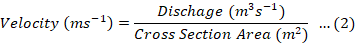
Velocities and discharges at each station were measured at fifteen-day intervals with the help of the SonTek YSI incorporation flow tracker. The mean section discharge equation and the procedure were adopted for discharge calculation as BS EN ISO 748 (2007) recommended. The water surface was divided into 0.5-meter ofssfsets, and velocities at each offset at a depth of 0.2, 0.6, and 0.8 were measured. The procedure is shown in Figure 4. The mean section discharge equation was used to calculatedischarges and flow cross-sectional area. The method is programmed in the flow tracker used in this research. The average velocity of the channel at the point was calculated using the following equation.

 

The SAW in the channel was comprised of Potamogeton perfoliatus, Hydrilla verticillate, Stuckenia pectinate, String Algae (Spirogyra spp.) and Vallisneria americana. After the data were checked for outliers, X-bar charts were created in SPSS Version.16 to guarantee the data’s quality. It is helpful to track the data process by using an X-bar chart. The illustrations make it easy to see mean changes. After determining the normalcy of all the data, the kind of analysis and correlation would be determined. Since none of the data was normally distributed, correlations were established using a quantal regression equation. A quantitative response variable is modeled by quantile regression using either qualitative or quantitative explanatory factors.

Koenker and Basset made the initial proposal for it in 1978 (Chen, 2007). Quantile regression was performed at quantile values of 0.25, 0.50, and 0.75 using Stata/MP 16.0. The best-suited model was selected based on the lowest Bayesian Information Criterion (BIC) and Akaike Information Criterion (AIC) values (Behl et al., 2014).

Results and Discussion

The measured monthly average SAW densities, the velocities, and the velocity cross-section profile temporally vary (Figure 5). With the increase of SAW densities, noticeable changes have occurred in the velocity’s cross-sectional profile. A clean profile was observed in July 2019 (Figure 5). The red-colored (0.4 ms-1) velocity contour decreased when the SAW growth began. It was found that the bottom velocity contour changes from 0.3 ms-1 to 0.2 ms-1 when the SAW channel grows. The flow velocity of 0.3 ms-1 to 0.2 ms-1 grew in size, whereas the contour for high velocity (0.4 ms-1) declined from July to December. It indicates that when vegetation grows, the flow concentrates in the cross-section where there is no vegetation and the velocity of the vegetated portion reduces. Figure 5 indicates that as the submerged aquatic weeds grew, the top velocity rose and the bottom velocity dropped. The results validate the findings of Li et al. (2014).

Descriptive statistics for average channel velocity and SAW densities are shown in Table 1. For all the parameters that were employed in the data modelling, there were 364 valid observations in total.

The minimum SAW densities have a zero value or no vegetation; the maximum velocity observed was 0.46 ms-1. The maximum velocity observed was lower than the designed velocity of 0.64 ms-1. The maximum SAW density observed was 247.33 kgm-3, while the corresponding minimum velocity was 0.16 ms-1. The mean SAW densities calculated for the overall season was 57.38 kgm-3, while the average velocity was 0.28 ms-1.

 

Table 1: Descriptive statistics of channel velocity and SAW densities.

	n	Minimum	Maximum	Mean	Std. Deviation
SAW densities (kgm-3)	364	0.00	247.33	57.38	54.63
Velocity (ms-1)	364	0.16	0.46	0.28	0.08

 

Table 2: Model for SAW densities and canal velocity.

Velocities		Coefficient	Bootstrap Std. Err.	t	P>│t│	[95% Conf. interval]
q25	SAWD	-0.0006	0.0001	-5.37	0.000	-0.0009	-0.0004
	Constant	0.2482	0.0070	34.98	0.000	0.2342	0.2621
q50	SAWD	-0.0003	0.0001	-2.93	0.004	-0.0005	-0.0001
	Constant	0.3030	0.0057	52.78	0.000	0.2917	0.3142
q75	SAWD	-0.0006	0.0001	-4.36	0.000	-0.0009	-0.0003
	Constant	0.3853	0.0190	20.19	0.000	0.3478	0.4228

 

Table 3: Model best-fit comparison for SAW densities and canal velocity.

Rank No.	Quantile	n	Sum of weights	DF	R²	Adjusted R²	AIC	BIC
1	q25	364	364	362	0.12	0.12	-1356.48	-1352.58
2	q75	364	364	362	0.13	0.13	-1320.34	-1316.44
3	q50	364	364	362	0.07	0.07	-1242.86	-1238.97

 

Table 2 shows parameters for 0.25, 0.50, and 0.75 quantiles relating channel velocity with SAW densities, while Table 3 shows the best-fit model comparison. Table 3 shows that 0.25 quantiles represent best-fit relationships of canal velocity with SAW densities . It can be observed from Table 2 that for the 0.25 quantile equation, SAW densities have significant negative relationships with a coefficient of 0.0006 and a constant value of 0.2482. The application of the bestfit model equation shows that when SAW densities are zero or there are no weeds in the channel, the channel velocity will be 0.2482 ms-1.

Conclusions and Recommendations

The study’s goal was to find out how submerged aquatic weed development affected channel velocity in the Dagai Distributary of the Upper Swat Canal irrigation system and to develop best fit model for velocity estimation. The results show that submerged aquatic weeds have a significant impact on channel velocity, as seen by variations in the cross-sectional velocity profile. The upper top velocity increased, and the bottom velocity decreased as the quantity of submerged aquatic weeds grew. A best-fit model for flow velocity in the vegetated channel was derived which is recommended for Dagai Distributary. To maintain desired flow conditions, the study suggests implementing management strategies for submerged aquatic vegetation, fsuch as periodic removal or control measures. Accurate forecasting and adaptive management of water channels will be facilitated by routine monitoring of channel velocity and submerged aquatic weed concentrations. To further confirm the results, it is suggested to do this sort of investigation in other geographic areas and canal systems.

Acknowledgements

We gratefully acknowledge the generous financial support provided for this research by the Higher Education Commission (HEC) of Pakistan. Their investment has been instrumental in enabling us to pursue our scientific inquiries and contribute to the advancement of knowledge in Water Management. We also extend our appreciation to WIT LUMS Lahore who have supported this work through their contributions and expertise.

Novelty Statement

In this research article equation for velocity calculation in a vegetative lined irrigation channel has been developed which is cite specific for Dagi Distributary.

Author’s Contribution

Jan Muhammad: Collected data, analyzed the data, and prepared the article.

Muhammad Zubair Khan: Developed the concept and supervised the research.

Haroon Khan: Supervised in field and data collection, manuscript writing and data analyses.

Conflict of interest

The authors have declared no conflict of interest.

References

Augustijn, D.C.M., F. Huthoff and E.H.V. Velzen. 2008. Comparison of vegetation roughness descriptions. Proc. River Flow 2008 Fourth Int. Conf. Fluv. Hydraul. Cesme, Turkey.

Behl, P., G. Claeskens and H. Dette. 2014. Focussed model selection in quantile regression. Stat. Sin., 24(2): 601–624. https://doi.org/10.5705/ss.2012.097

Boothroyd, R.J., R.J. Hardy, J. Warburton and T.I. Marjoribanks. 2016. The importance of accurately representing submerged vegetation morphology in the numerical prediction of complex river flow. Earth. Surf. Process. Landf., 41(4): 567-576. https://doi.org/10.1002/esp.3871

BS EN ISO 748. 2007. Hydrometry- Measurement of liquid flow in opened channels using current meters of floats. 3: 46.

Chen, C., 2007. A finite smoothing algorithm for quantile regression. J. Comput. Graph. Stat., 16(1): 136-164. https://doi.org/10.1198/106186007X180336

Cheng, L. and Y.M. Shen. 2008. Flow structure and sediment transport with impacts of aquatic vegetation. J. Hydrodyn., 20(4): 461–468. https://doi.org/10.1016/S1001-6058(08)60081-5

Defina, A. and A.C. Bixio. 2005. Mean flow and turbulence in vegetated open channel flow. Water Resour. Res., 41(7): 1–12. https://doi.org/10.1029/2004WR003475

Green, J.C., 2005. Velocity and turbulence distribution around lotic macrophytes. Aquatic Ecol., 39(1): 1-10. https://doi.org/10.1007/s10452-004-1913-0

GU, F., N.I. Han and Q.I. Ding. 2007. Roughness coefficient for unsubmerged and submerged reed. J. Hydrodyn., 19: 421-428. https://doi.org/10.1016/S1001-6058(07)60135-8

Huai, W.X., Y.H. Zeng, Z.G. Xu and Z.H. Yang. 2009. Three-layer model for vertical velocity distribution in open channel flow with submerged rigid vegetation. Adv. Water Resour., 32(4): 487–492. https://doi.org/10.1016/j.advwatres.2008.11.014

IWMI, 2011. Post-project evaluation of pehur high level canal (PHLC) project final report. Lahore, Pakistan.

Jalonen, J., 2015b. Hydraulics of vegetated flows: Estimating riparian plant drag with a view on laser scanning applications. Ph. D thesis, department of civil and environmental engineering, Aalto University, Finland.

Jalonen, J., J. Järvelä and J. Aberle. 2013. Leaf area index as vegetation density measure for hydraulic analyses. J. Hydraul. Eng. ASCE. pp. 461–469. https://doi.org/10.1061/(ASCE)HY.1943-7900.0000700

Jalonen, J., J. Jarvela, J.P. Virtanen, M. Vaaja, M. Kurkela and H. Hyyppa. 2015a. Determining characteristic vegetation areas by terrestrial laser scanning for floodplain flow modelling. Water (Switzerland). 7(2): 420-437. https://doi.org/10.3390/w7020420

Klopstra, D., H.J. Barneveld, J.M. Van Noortwijk and E.H. Van Velzen. 1997. Analytical model for hydraulic roughness of submerged vegetation. Proc. Congr. Int. Assoc. Hydraul. Res. IAHRA (3): 775-780.

Lawrence, J.M., 1966. Aquatic weed control in fish ponds. FAO Fish. Rep., 44(5): 76–91.

Li, Y., Y. Wang, D.O. Anim, C. Tang, W. Du, L. Ni, Z. Yu and K. Acharya. 2014. Flow characteristics in different densities of submerged flexible vegetation from an open-channel flume study of artificial plants. Geomorphology, 204: 314-324. https://doi.org/10.1016/j.geomorph.2013.08.015

Lopez, F. and M.H. Garcıa. 2007. Flow patterns of oil water gas three-phase downward flow and transition from bubble flow to slug flow. J. Hydraul. Eng. © ASCE: 392–402.

McKenzie, L.J., S.J. Campbell and C.A. Roder. 2001. Seagrass watch: A manual for mapping and monitoring seagrass resources by community (citizen) volunteers. QFS, NFC, Cairns, 1: 94.

O’Hare, M.T., C. McGahey, N. Bissett, C. Cailes, P. Henville and P. Scarlett. 2010. Variability in roughness measurements for vegetated rivers near base flow, in England and Scotland. J. Hydrol., 385: 361-370. https://doi.org/10.1016/j.jhydrol.2010.02.036

Samani, J.M.V. and M. Mazaheri. 2009. An analytical model for velocity distribution in transition zone for channel flows over inflexible submerged vegetation. J. Agric. Sci. Technol., 3(11): 25–33.

Stone, B.M. and H.T. Shen. 2002. Hydraulic resistance of flow in channels with cylindrical roughness. J. Hydraul. Eng., 128(5): 500–506. https://doi.org/10.1061/(ASCE)0733-9429(2002)128:5(500)

Verschoren, V., D. Meire, J. Schoelynck, K. Buis, K.D. Bal, P. Troch, P. Meirem and S. Temmerman. 2016. Resistance and reconfiguration of natural flexible submerged vegetation in hydrodynamic river modelling. Environ. Fluid Mech., 16: 245-265. https://doi.org/10.1007/s10652-015-9432-1

Weiming, W.U. and H.E. Zhiguo. 2009. Effects of vegetation on flow conveyance and sediment transport capacity. Int. J. Sediment Res., 24(3): 247–259. https://doi.org/10.1016/S1001-6279(10)60001-7