Research Article

Estimation of Net Rice Production by Remote Sensing and Multi Source Datasets

Syed Muhammad Hassan Raza1*, Syed Amer Mahmood1, Syeeda Areeba Gillani1, Syed Shehzad Hassan1, Muneeb Aamir1, Muhammad Saifullah1, Mubashar Basheer1, Atif Ahmad1, Saif-ul-Rehman2 and Tariq Ali1

1RS/GIS group, Space Science Department, Punjab University Lahore, Pakistan; 2Department of Geography Government College University Lahore.

Received | November 04, 2018; Accepted | August 15, 2019; Published | September 12, 2019

*Correspondence | Syed Muhammad Hassan Raza, RS/GIS group, Space Science Department, Punjab University Lahore; Email: [email protected]

Citation | Raza, S.M.H., S.A. Mahmood, S.A. Gillani, S.S. Hassan, M. Aamir, M. Saifullah, M. Basheer, A. Ahmad, S. Rehman and T. Ali. 2019. Estimation of net rice production by remote sensing and multi source datasets. Sarhad Journal of Agriculture, 35(3): 955-965.

DOI | http://dx.doi.org/10.17582/journal.sja/2019/35.3.955.965

Keywords | RVI, NDVI, Ratio Vegetation Index (RVI), Crop Reporting Service (CRS), Linear regression, Yield estimation

Introduction

Rice is among three leading crops of the world with wheat and maize which is largely grown and widely used. Nearly 88% of the global rice is cultivated in Asian countries (Mostafa et al., 2016; Behzad et a., 2019), where 2.4 billion population intake rice as regular food. According to recent estimates, China was the leading country with 211 million tons of rice production throughout the world (Raza et al., 2018a). The rice area is decreasing due to fastest growth in urbanization (Gillani et al., 2019) that occurred in recent decades. This urbanization has eaten up very fertile rice lands while the rice demands is expected to be 875m tons up to 2030 (Huang et al., 2002). Rice cultivation is dependent upon a variety of parameters including crop phonology, anthropogenic activities and physician characteristics of soil (Raza et al., 2018b).

A worldwide survey authenticates that 87% of rice farms are under cultivation by individuals who have small lands (Nagayet, 2005). These cultivators face big challenges to achieve targeted yield e.g., worst weather events, pest attacks, water stress (Saifulla et al., 2019) and the market fluctuations in term of income security (Morton, 2007; O’Brien et al., 2004). Other hostile scenarios like, uneven distribution of rainfall, glacial retract and a rise in sea level, droughts and storm surges are the main reasons to intensify the risks of yield degradations (Parry et al., 2007). Asian countries are commonly affected by these climatic events (Mendelsohn, 2009). The abruptly changing environment (Hassan et al., 2019) has applied a huge pressure on small farmers to produce healthy to cater the demands of masses (Raza, 2018c). Therefore, it is significant to predict the net production that make capable to agronomists to estimate the exact quantity that can be imported or exported. This technique is good to tackle food crisis well in time (Sandhu et al., 2019). Yield estimation is therefore viable to eliminate the impact of these challenges by reducing production losses and increasing per hector yield (Mindra, 2011; Shannon, 2015; Raza, 2018a; Swain, 2014). Estimation of area yield has become a challenging factor to achieve promised yield therefore it is attractive to agri-industry and farmers (Miranda, 2011). AYIC is based on historic crop yield records. The availability of historic crop related datasets is limited in rice producing countries like Pakistan, India and Bangladesh etc. that is a constrain to implement AYIC (Miranda, 2012). Historic datasets regarding crop production, are of great importance due to their unbiased and replicable nature that are used to achieve accurate yield by their integration with remote sensing data (Fang et al., 2008).

There are many methods available to evaluate the rice yield but the most commonly used method is to generate a relationship of rice crop response and the historical yields. The main theme is creation of relation of yield with crop photosynthesis capacity. NDVI and RVI verifies that the amount of photosynthetic activity is responsible for biomass generation and is captured by spectral responses (Prasad et al., 2007).

In Pakistan, field surveys are conducted by field officers in their area of commands in collaboration with staff of CRS department as a joint venture of irrigation and agriculture department. Final estimates are approved by Agriculture, Irrigation, P&D and Revenue departments and are made public after the crop cultivation.

This research aim at evaluating the net rice production for upcoming year 2019 using historic crop related records saved by Punjab CRS department in collaboration with open source satellite imagery. It also aimed at describing the efficiency and reliability of satellite images in comparison to ancient ways of crop monitoring using a large man power with wastage of time.

Materials and Methods

Study site

The investigation site consists of major rice yielding regions of Punjab province in Pakistan including Lahore, Sheikhupura, Nankana Sahib, Gujranwala and Hafizabad. The investigation site is famous around the world to produce high quality of rice. This region fall on the way of monsoon therefore, it receives a large amount of rainfall which is more than 500 mm. The map of study area is drawn in Figure 1.

Experimental design

The “Step by Step” methodology is mapped in Figure 2. In the first step we downloaded satellite images as captured by various Landsat satellites for the duration from 2008 to 2018 and computed NDVI and RVI values for each year. The area/yield records related to rice crop as preserved by CRS department were also acquired. The regression analysis applied to satellite compute and the CRS reported yield values and generated regression equations. These regression equations were further used to compute rice yield because these equations are showing a trend. We used supervised classification for estimation of rice area precisely. The flow of research is mentioned in Figure 2.

Yield estimation through field surveys by interviewing farmers is commonly used worldwide. In this method, the field trips are conducted seasonally for each cluster site throughout the country. Agronomists along with field staff, surveyed all plots many time for monitoring all crop growth/yield limiting parameters e.g., light use efficiency, insect’s activity and the water intake level by a particular crop (Motha, 2015). The computed parameters are essential to compute per hector yield.

Consecutive filed surveys are also used as an alternative method of crop monitoring and yield estimation by selecting some sites (Swain, 2014). The results obtained through these sites are used as primary data and are applied to the whole study site to estimate the crop yield (Bala et al., 2008). This technique of estimation of yield may result into various drawbacks such as, it is cost effective and time-consuming method, the outcomes are shared after many months of harvest of a crop that is not usable at that time (Noureldin et al., 2013). This mechanism has no ability to cover large areas efficiently.

In comparison to above discussed methods of yield estimation, remote sensing provides real time, georeferenced temporal datasets which are highly reliable and easy to handle. These datasets are widely used throughout the world to predict the crop yield and to map crop area accurately (Rahman et al., 2009). Satellite technology can give efficient results because it provides pixel-based information for large geographies. The satellite imagery is available sometime free (i.e., Landsat and MODIS etc.) and the large areas are covered with high temporal resolution.

Various spectral bands mounted in satellites are capable to record the spectral reflectance of crop canopies which can be used to monitor crop health. (Gortan, 1993; Hunge et al., 2013; Rahman et al., 2009). Biomass generation of each day can be evaluated using temporal responses of these spectral bands. The combinations of spectral bands are useful to apply vegetative indices for estimation of crop related parameters. The vegetative indices were developed to compare red and infrared bands because maximum chlorophyll absorption occur in visible band as compared to maximum reflection in NIR (Lee et al., 2000).

RVI is a vegetative index used to highlight vegetation as compared to other feature e.g., soil, snow or water. However, the NDVI is commonly used to determine the spectral responses for rice crop. NDVI and RVI are computed using Equations 1 and 2 (Bunkei Matsushita et al., 2007; Nabi et al., 2019).

 

 

We acquired open source imagery (Landsat data) from United States Geological Survey (USGS) of the complete duration, mentioned in Table 1, 2. Most of Landsat imagery is comprised with pixel size of 30m and a 16 days temporal window (Jeffery et al., 2001).

Table 1: Image acquisition dates of Landsat 5,7 along with solar angle, quantized calibrated digital number and the total spectral radiance of Band 3 and Band 4.

S. No	Satellite	Date	Band 3	Band 4	Band 3	Band 4	Solar Angle θ
1	Landsat 5	23-Jul-08	264	221	-1.17	-1.51	63.24
2	Landsat 5	25-Sep-08	264	221	-1.17	-1.51	50.33
3	Landsat 5	28-Nov-08	264	221	-1.17	-1.51	32.57
4	Landsat 5	10-Jul-09	264	221	-1.17	-1.51	65.05
5	Landsat 5	12-Sep-09	264	221	-1.17	-1.51	54.66
6	Landsat 5	15-Nov-09	264	221	-1.17	-1.51	30.59
7	Landsat 5	27-Jun-10	264	221	-1.17	-1.51	66.41
8	Landsat 5	30-Aug-10	264	221	-1.17	-1.51	57.89
9	Landsat 5	2-Nov-10	264	221	-1.17	-1.51	39.61
10	Landsat 5	1-Aug-11	264	221	-1.17	-1.51	62.71
11	Landsat 5	18-Sep-11	264	221	-1.17	-1.51	53.02
12	Landsat 5	13-Nov-2011	264	221	-1.17	-1.51	36.99
13	Landsat 7	10-Jul-12	234	241	-5	-5	66.25
14	Landsat 7	28-Sep-12	234	241	-5	-5	50.86
15	Landsat 7	15-Nov-12	234	241	-5	-5	36.48

 

Table 2: Image acquisition dates of Landsat 8 along with multiband reflectance of Band 4 and Band 5.

	Satellite		Reflectance Multiband B4	Reflectance Additive B4	Reflectance Multiband B5	Reflectance Additive B5	Solar Elevation θ
16	Landsat 8	19-Jun-13	0.00002	-0.1	0.00002	-0.1	68.65
17	Landsat 8	23-Sep-13	0.00002	-0.1	0.00002	-0.1	53.19
18	Landsat 8	26-Nov-13	0.00002	-0.1	0.00002	-0.1	34.46
19	Landsat 8	22-Jun-14	0.00002	-0.1	0.00002	-0.1	68.62
20	Landsat 8	26-Sep-14	0.00002	-0.1	0.00002	-0.1	52.29
21	Landsat 8	29-Nov-14	0.00002	-0.1	0.00002	-0.1	33.82
22	Landsat 8	25-Jun-15	0.00002	-0.1	0.00002	-0.1	68.35
23	Landsat 8	29-Sep-15	0.00002	-0.1	0.00002	-0.1	51.28
24	Landsat 8	2-Dec-15	0.00002	-0.1	0.00002	-0.1	33.33
25	Landsat 8	27-Jun-16	0.00002	-0.1	0.00002	-0.1	68.43
26	Landsat 8	1-Oct-16	0.00002	-0.1	0.00002	-0.1	50.46
27	Landsat 8	4-Dec-16	0.00002	-0.1	0.00002	-0.1	32.88
28	Landsat 8	14-Jun-17	0.00002	-0.1	0.00002	-0.1	68.42
29	Landsat 8	18-Sep-17	0.00002	-0.1	0.00002	-0.1	52.22
30	Landsat 8	21-Nov-17	0.00002	-0.1	0.00002	-0.1	31.78
31	Landsat 8	1-Jun-18	0.00002	-0.1	0.00002	-0.1	67.85
32	Landsat 8	5-Sep-18	0.00002	-0.1	0.00002	-0.1	50.82
33	Landsat 8	8-Nov-18	0.00002	-0.1	0.00002	-0.1	31.12

The image acquisition dates were according to the rice growth duration e.g., germination, transplantation, panicle primordia initiation, milky dough and the harvest stages (Mkhabela et al., 2011). The species other than rice were observed less than 1% in various field surveys. The complete information of downloaded images is listed in Table 1 and Table 2.

Scan Line Corrector (SLC) of Landsat 7 stopped working on May 31, 2003 that resulted in missing strips. A complete scene of Swath with 185 km2 had 22% data missing. The missing data was recovered by comparing it with natural imagery using nearest neighborhood techniques.

Geometric corrections are related to the variations in spatial location of various features mapped by satellite imagery in comparison to their actual positions on the surface of earth. Geometric corrections are significant to perform to cross match the geographic locations of various features in satellite image with real world. For this, we demarcated major features e.g., river crossings the GT road with actual locations using differential global positioning system.

TOA calculation provides noise free datasets to obtain accurate results. TOA calculations give more appropriate results in comparison to the method of atmospheric corrections. The algorithm of TOA calculation is not similar for all the satellite e.g., The TOA generation for Landsat 5, 7 is described in Equations 3 and 4.

 

 

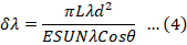
Where the parameters in Equation 3, 4 are tracked from metadata attached to a particular image and spectral radiances are denoted as Lmax and Lmin. Qmax and Qmin are quantized calibrated digital number and L is the total spectral radiance recorded in watt/m2. In Equation 4 δλ is TOA reflectance Esun is exo-atmospheric irradiance, Lλ is the spectral radiance at the sensor’s aperture [W∕ðm2 sr μm], d is the distance of earth from sun, π is the constant having value 3.14 and θ is solar elevation recorded in decimal degreed.

The specific method to compute TOA reflectance for Landsat 8 is mentioned Equations 5, 6.

 

 Table 3: District wise area and yield values as reported by CRS for the years 2008-2018.

Years	2008	2008	2009	2009	2010	2010	2011	2011	2012	2012	2013	2013
District	Area (ha)	Yield (ton/ha)	Area (ha)	Yield (ton/ ha)	Area (ha)	Yield (ton/ha)	Area (ha)	Yield (ton/ ha)	Area (ha)	Yield (ton /ha)	Area (ha)	Yield (ton /ha)
Lahore	43800	1.90	34000	1.85	32800	1.81	32000	1.74	28700	2.26	38030	1.88
Gujran- wala	249200	1.99	248000	2.21	241200	2.1	249300	2.2	247300	2.33	248880	2.19
Hafiza- bad	130300	1.89	133000	2.1	127100	2.1	126300	1.99	271900	2.11	132740	2.25
Nankana Sb	114600	1.84	102000	1.80	96300	1.8	97500	1.79	96300	1.94	103600	2.22
Sheikh-upura	184500	1.68	206000	1.80	202300	1.7	206800	1.78	205600	1.71	196270	1.97
Total Area	722400		723000		699700		711900		706600		719520
Average Yield		1.86		1.95		1.9		1.89		2.07		2.012
Years	2014	2014	2015	2015	2016	2016	2017	2017	2018	2018
District	Area (ha)	Yield (ton/ha)	Area (ha)	Yield (ton/ ha)	Area (ha)	Yield (ton/ha)	Area (ha)	Yield (ton /ha)	Area (ha)	Yield (ton /ha)
Lahore	40470	2.15	34800	2.08	32380	1.96	31960	1.98	34000	1.95
Gujran- wala	238360	2.18	225000	2.35	222570	2.36	220950	2.21	226620	2.09
Hafiz- abad	123020	2.12	133550	2.30	133540	2.33	129000	2.62	136370	2.34
Nankana Sb	108860	2.25	112100	2.12	106420	2.16	102790	2.2	111690	2.17
Sheikh- upura	200310	1.96	172390	2.13	171180	2.04	171180	2.0	180900	2.07
Total Area	711020		677840		666090		655880		689580
Average Yield		2.13		2.19		2.092		2.2		2.12

 

 

Where;

θ is the solar angle in Equations 5, 6 and other factors were obtained from metadata of Landsat 8 images.

Crop related historical datasets saved by CRS department are of great importance. We obtained area under rice cultivation in km2 and the annual rice yield for the years 2008 to 2018 as published by CRS department in Table 3.

A 15-band composite was generated by applying layer stack utility e.g., the 15-band composite for the year 2008 was composed with (5 spectral bands obtained using satellite image of 2008, 5 of September and November 2008). Figure 3 is showing the composite scheme consist of 15 spectral bands. This composite provides efficient classification results because this composite provides the integrated impact of all stages of rice plant growth.

The strategy developed in Figure 3 was applied on both satellite systems Landsat 5, 7 and Landsat 8. In case of Landsat 5, 7, we used bands 1-5 covering the visible and infrared wavelengths of electromagnetic spectrum. Similarly, we used Bands 2-6 of Landsat 8 in visible and infrared wavelength ranges to develop the 15 Bands composite as described in Figure 3.

The predicted values in comparison to actual values are well defined by RMSE. In this research, the historical datasets are the observed values. Mathematically, where Pi and Oi are predicted and observed values respectively. The value of RMSE is ideal (Siyal et al., 2015).

 

The underestimation or overestimation in datasets can be predicted by MBE. It is an efficient tool to determine biasness in the input data. A negative MBE describe the amount of underestimation for predicted values. Mathematically (Siyal et al., 2015).

 

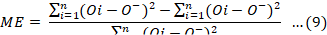
ME give the integrated impact of RMSE and MBE that defines the accuracy in a model. Mathematically (Willmott, 1982).

 

Results and Discussion

The spectral bands in NIR and Red wavelengths of Landsat 5,7 and 8 are selected to calculate NDVI and RVI values. We selected the images of September only because the highest NDVI and RVI values can be achieved in September. TOA based datasets were obtained by converting pixel based DN values of all spectral datasets using Equations 3 and 4 for Landsat 5,7 and the Equations 5 and 6 for Landsat 8. We computed annual variations in NDVI and RVI values and listed the results in Table 4. The annual yield values acquired from CRS Punjab department from 2008-2018 are also listed in the Table 4.

Table 4: RVI and NDVI values recorded in September for the years 2008-2018 to compute the CRS based yield.

S. No.	Date	NDVI	RVI	CRS based Yield
1	25-Sep-08	0.67	3.63	1.86
2	12-Sep-09	0.69	4.02	1.95
3	30-Aug-10	0.66	3.52	1.9
4	18-Sep-11	0.68	3.49	1.89
5	28-Sep-12	0.72	4.16	2.07
6	23-Sep-13	0.71	3.97	2.012
7	26-Sep-14	0.73	4.4	2.13
8	29-Sep-15	0.74	4.65	2.19
9	15-Sep-16	0.76	4.62	2.12
10	18-Sep-17	0.73	4.75	2.2
11	5-Sep-18	0.72	4.76	2.05

The linear regression applied to CRS yield records against NDVI values is mentioned in Figure 4. Figure 4 is showing a strong relation between these variables having a coefficient of determine R2= 0.8239.

We generated an equation to compute NDVI based yield for coming years.

 

Similarly, a regression analysis of CRS based yield with RVI values is mapped in Figure 5. A regression equation was also generated as Equation 11, which shows a fair relationship between RVI values and the annual yield having R2= 0.817.

 

The satellite derived yield values were computed as mentioned in Table 5.

Table 5: Yield estimation using satellite datasets for the years 2008-2018 using annual NDVI and RVI values.

Date	NDVI	RVI	Yield (ton/ha) using NDVI	Yield (ton/ha) using RVI
25-Sep-08	0.67	3.63	1.89	1.91
12-Sep-09	0.69	4.02	1.96	2.00
30-Aug-10	0.66	3.52	1.86	1.89
18-Sep-11	0.68	3.49	1.93	1.88
28-Sep-12	0.72	4.16	2.07	2.03
23-Sep-13	0.71	3.97	2.03	1.99
26-Sep-14	0.73	4.4	2.10	2.08
29-Sep-15	0.74	4.65	2.14	2.14
15-Sep-16	0.76	4.62	2.21	2.13
18-Sep-17	0.73	4.75	2.10	2.16
5-Sep-18	0.72	4.76	2.07	2.16

The regression analysis of both yield values (RVI and NDVI based) is mapped in Figure 6 which were found in strong correlation with R2 = 0.7882. This values of R2 allow us to choose an Equation 10 or 11 for estimation of yield for 2019 but we proceeded our task with Equation 10 due to high interactivity, reliability and global coverage/usage of NDVI. This index in depth while RVI is commonly used to delineate vegetation in comparison to other features e.g., water, snow or soil textures.

Estimation of rice area

To delineate the rice areas for the years 2008 to 2018, the algorithm of supervised classification was applied. Supervised classification is not capable to discriminate between various species such as grass and crop which consider grass in account of crop areas. A satellite image was obtained which recorded the study site just before the germination of rice. This image highlighted the species other than rice and were considered as non-rice areas. The weightage of these non-rice areas was less than 1% which was subtracted to estimate the exact extent of rice plantations in km2. The rice cultivations were extracted using supervised classification is mapped in Figure 7.

Figure 7 is showing the 11-sample site using satellite imageries to map the rice area for the complete study period, where the green area represents the rice crop whereas the light/dark blue are is showing non rice features e.g., water and the human settlements in the study site.

The CRS reported rice areas were compared with satellite derived areas. The satellite derived area was in exaggeration in comparison to actual areas which represents that the Landsat imagery had coarse resolution which may incorporate the rice cropping along roads in account of features other than vegetation. However, other high-resolution datasets e.g., the products of world-view, Quick bird and Geo-Eye provide improved classification results however, these imageries may result in big economical cost for such large areas more than 75000 ha. Satellite derived areas along with CRS areas are drawn in the Figure 8.

The result of linear regression applied to CRS reported rice area in comparison to satellite derived area are shown in Figure 9 that presents a strong relationship with coefficient of determination R2=0.844 and generated an equation as below,

 

The accuracy of this model was estimated through three statistical indicators. The results determine a fair relationship between compute and estimated rice areas with ME=0.95, MBE=0.86 AND RMSE=0.67. These ME, MBE and RMSE reveal that the computed records corresponds to the predicted records.

The rice plant undergoes three sequential stages including vegetative stage, reproductive stage and the ripening stage. These stages are further subdivided into germination, seedling, leaf emergence, transplantation, panicle primordia initiation, heading/anthesis and ripening stage. In germination, the embryo of rice seed germinates by heat and moisture content and the white tip appears from the surface of land or water. The germination process is highly dependent upon the environmental conditions and drawing the nutrients from soil or air. We observed various growth rates for germinations stage in the study site. The plots bearing a temperature range between 30-35 oC were early germinated in comparison to the plots bearing 20 oC. Leaf emergence is the next process which was observed highly dependent upon the temperature e.g., a leaf takes about 100-degree days for its full emergence therefore, a rice plant bearing 20 oC will produce a leaf on every 5th day and a plant bearing 20 oC will produce a leaf on every 4th day. The branches are known as tillers which emerge from second leaf of main culm as it emerges 5th leaf on main culm. The initialization of panicle is known as heading/anthesis. We observed that the heading stage took about 15-18 days in the study site. The heading stage was observed high dependent upon temperature, as a difference of 1oC caused a delay about 14 days. The ripening stage is considered the final stage in which the milky dough ripes and turn to yellow then white. The ripening stage needs comparatively low temperature as compared to other growth stages. We observed the rice plant in the basis three growth stages and computed the variations in NDVI using satellite spectral bands throughout the life period and mapped the results in Figure 10.

Net rice production in 2018

We used a satellite image of Landsat 8 to delineate the rice area in the study site. Supervised classification of this image represents that 689580 ha of area was under rice cultivation in 2018. To cross validate the classification results, we visited the study site physically with Malli Patwari (A person who has all the information regarding the area under cultivation in his area of command), using Global Positioning System (GPS). We pointed out some remote locations on the map which were not easily recognized which were identified closer to urban areas. The GPS based ground survey determined the precision of classification about 89% that can be 92% (Sisodia et al., 2014). The satellite extracted rice area was put in Equation 12 to estimate the rice area as per CRS records that was 654966 ha. The rice yield was predicted using NDVI value of the year 2018 which results as 0.72. This NDVI value was placed in Equation 10 to compute the yield which 2.05 ton/ha. The total rice production was obtained by a product of CRS based area (654966 ha) with the predicted yield (2.08 ton/ha) that was 1.42 m ton of rice. Same methodology was used by various authors e.g., (Karamat et al., 2019; Siyal et al., 2015) used the same methodology to compute the rice yield.

Conclusions and Recommendations

This study emphasis the reliability of historic data sets to predict rice yield. This project is actually the joint venture of historic records with satellite imagery. The technique that we used in this research to compute the net rice production is handy to apply anywhere, even in complex ecological conditions. It can assist decision makers and agronomists to estimate crop volume well in time before harvest to determine the exact amount of import/export.

Acknowledgement

We are thankful to United States Geological Survey (USGS) for providing us their valuable data to complete this research.

Author’s Contribution

Syed Muhammad Hassan Raza provided complete supervision of the project, helped in data processing and planning in surveys. Syed Amer Mehmood arranged funds to conduct field surveys, helped in writing the manuscript and complete supervision of the project virtually. Syed Shehzad Hassan did data collection, processing and complete supervision. Muhammad Saifullah performed data acquisition, statistical analysis and data finalization. Syeda Areeba Gillani scientific proof reading and removal of grammatical mistakes from the manuscript. Muneeb Aamir did data processing, field visit and monitoring the technicalities of field Surveys. Mubashar Basheer did data collection and data processing and Atif Ahmad, Filed surveys and ground truthing. Tariq Ali and Saif-ul-Rehman contributed in phenological stages of rice and plotting their spectral response.

Novelty Statement

We confirm that the information added in manuscript is original and novel. It will provide a new technique to researchers and farmers which is simple and applicable anywhere.

References

Karamat, A., A. Rehman, M. Ayyaz, S. Ali, I. Manzoor, A.H. Ashraf, F. Riaz, M.U. Tanveer and S.A. Mahmood. 2019. Estimation of net rice production for the fiscal year 2019 using multisource datasets. Int. J. Agric. Sustainable Dev. Vol 01. Issue 02: pp. 47-65.

Bala, S.K. and A.K.M.S. Islam. 2008. Estimation of potato yield in and around munshiganj using remote sensing ndvi data. Inst. Water Flood Manage. Dhaka, Bangladesh. p. 79.

Behzad, A., U. Rafique, M. Qamar, B. Islam, H. Umer, U.H. Hameed, M. Basheer, M. Firdos and S.A. Mahmood. 2019. Estimation of net primary production of rice crop using casa model in Nankana Sahib. Int. J. Agric. Sustainable Dev. Vol 01, Issue 01: pp. 30-46. https://doi.org/10.33411/IJASD/2019010103

Matsushita, B., W. Yang, J. Chen, Y. Onda and G. Qiu. 2007. Sensitivity of the Enhanced Vegetation Index (EVI) and Normalized Difference Vegetation Index (NDVI) to topographic effects: A Case Study in High-Density Cypress Forest” sensors.7: 2636-2651. https://doi.org/10.3390/s7112636

Willmott, C.J. 1982. Some comments on the evaluation of model performance. Bull. Am. Meteorol. Soc. 63(11): 1309–1313. https://doi.org/10.1175/1520-0477(1982)063<1309:SCOTEO>2.0.CO;2

Fang, H., S. Liang, G. Hoogenboom, J. Teasdale and M. Cavigelli. 2008. Corn-yield estimation through assimilation of remotely sensed data into the CSM-CERES-Maize model. Int. J. Remote Sens. 29 (10): 3011–3032. https://doi.org/10.1080/01431160701408386

Gillani, S.A., S. Rehman, H.H. Ahmad, A. Rehman, S. Ali, A. Ahmad, U. Junaid and Z.M. Ateeq. 2019. Appraisal of urban heat island over Gujranwala and its environmental impact assessment using satellite imagery (1995-2016). Int. J. Innov. Sci. Technol. Vol. 01, Issue 01: pp. 1-14. https://doi.org/10.33411/IJIST/2019010101

Groten, S.M.E. 1993. NDVI Crop Monitoring and Early Yield Assessment of Burkina-Faso. Int. J. Remote Sens. 14: 1495–1515. https://doi.org/10.1080/01431169308953983

Hassan, S.S., M. Mukhtar, U.H. Haq, A. Aamir, M.H. Rafique, A. Kamran, G. Shah, S. Ali and S.A. Mahmood. 2019. Additions of tropospheric ozone (O3) in regional climates (A case study: Saudi Arabia). Int. J. Innov. Sci. Technol. Vol. 01, Issue 01: pp. 33-46. https://doi.org/10.33411/IJIST/2019010103

Huang, J.X., X. Wang, H. Li and Z. Tian. 2013. Remotely sensed rice yield prediction using multi-temporal NDVI data derived from NOAA’s AVHRR. PLoS One. 8: e70816. https://doi.org/10.1371/journal.pone.0070816

Huang, J.F., T. Shu-chuan, O. Abou-Ismail and W. Ren-chao. 2002. Rice yield estimation using remote sensing and simulation. J. Zhejiang Univ. Sci. A 3(4): 461–466. https://doi.org/10.1631/jzus.2002.0461

Jeffrey, G., Masek, M. Honzak, S.N. Goward, P. Liu and E. Pak. 2001. Landsat-7 “ETM+ as an observatory for land cover Initial radiometric and geometric comparisons with Landsat-5 Thematic Mapper. Remote sens. Environ. 78(1): 118-130. https://doi.org/10.1016/S0034-4257(01)00254-1

Lee, R., D. Kastens, K. Price and E. Martinko. 2000. Forecasting corn yield in Iowa using remotely sensed data and vegetation phenology information. January 10–12; Lake Buena Vista, Florida. 460–467.

Mkhabela, M.S., P. Bullock, S. Raj, S. Wang and Y. Yang. 2011. Crop yield forecasting on the Canadian Prairies using MODIS NDVI data. Agric. For. Meteorol. 151: 385–393. https://doi.org/10.1016/j.agrformet.2010.11.012

Miranda, M.J. and K. Farrin. 2012. Index insurance for developing countries. Appl. Econ. Perspect. 34 (3): 391–427. https://doi.org/10.1093/aepp/pps031

Mendelsohn, R. 2009. The impact of climate change on agriculture in developing countries. J. Nat. Resour. 1(1): 5–19. https://doi.org/10.1080/19390450802495882

Miranda, M.J., and C. Gonzalez-Vega. 2011. Systemic risk, index insurance, and optimal management of agricultural loan portfolios in developing countries. Am. J. Agric. Econ. 93(2): 399–406. https://doi.org/10.1093/ajae/aaq109

Motha, R.P. 2015. Managing weather and climate risks to agriculture in North America, Central America and the Caribbean. Weather Climate Extremes, 10(1): 50–56.

Morton, J.F., 2007. The impact of climate change on smallholder and subsistence agriculture. Proc. Natl. Acad. Sci. 104(50) 19680-19685.

Mostafa, K., Malesh, K. Quazi, Hassan, H. Ehsan and Chowdhury. 2016. Development of Remote Sensing Based Rice Yield Forecasting Model. Spanish J. Agric. Res. 14(2). https://doi.org/10.5424/sjar/2016143-8347

 Nabi, G., I.S. Kaukab, S.S.A.S. Zain, M. Saif, M. Malik, Nazeer, N. Farooq, R. Rasheed and S.A. Mahmood. 2019. Appraisal of deforestation in district Mansehra through Sentinel-2 and Landsat imagery. Int. J. Agric. Sustainable Dev. Vol. 01, Issue 01: pp. 1-16. https://doi.org/10.33411/IJASD/20190102

Noureldin, N.A., M.A. Aboelghar, H.S. Saudy and A.M. Ali. 2013. Rice yield forecasting models using satellite imagery in Egypt. Egypt. J. Remote Sens. Space Sci. 16: 125–131. https://doi.org/10.1016/j.ejrs.2013.04.005

Nagayet, O. Small Farms, Current Status and Key Trends. 2005. In the future of small farms, proceedings of a research workshop, Wye, UK, 26–29 June; Int. Food Policy Res. Inst. Washington, DC. USA. pp. 355–367.

Sandhu, N. and A. Kumar. 2017. Bridging the rice yield gaps under drought: QTLs, Genes, and their use in breeding programs. Agron. 7(2): 27. https://doi.org/10.3390/agronomy7020027

Sandhu, N., R.B. Yadaw, B. Chaudhary, H. Prasai, K. Iftekharuddaula, C. Venkateshwarlu, A. Annamalai, P. Xangsayasane, K.R. Battan, M. Ram, M.T.S. Cruz, P. Pablico, P.C. Maturan, K.A. Raman, M. Catolos and A. Kumar. 2019. Evaluating the performance of rice genotypes for improving yield and adaptability under direct seeded aerobic cultivation conditions. Front. Plant Sci. 10: 159.

O’Brien, K., R. Leichenko, U. Kelkar, H. Venema, G. Aandahl, H. Tompkins, A. Javed, S. Bhadwal, S. Barg, L. Nygaard, J. West. 2004. Mapping vulnerability to multiple stressors: Climate change and globalization in India. Glob. Environ. Change. 14(4): 303–313. https://doi.org/10.1016/j.gloenvcha.2004.01.001

Parry, M.L., O.F. Canziani, J.P. Palutikof, P.J. van der Linden, C.E. Hanson. 2007. Impacts, adaptation and vulnerability. contribution of working group ii to the fourth assessment report of the intergovernmental panel on climate change. Cambridge Univ. Press. Cambridge, UK,

Prasad, A.K., R.P. Singh, V. Tare and M. Kafatos. 2007. Use of vegetation index and meteorological parameters for the prediction of crop yield in India. Int. J. Remote Sens. 28: 5207–5235. https://doi.org/10.1080/01431160601105843

Rahman, A., L. Roytman, N.Y. Krakauer, M. Nizamuddin and Goldberg. 2009. M. Use of vegetation health data for estimation of Aus rice yield in Bangladesh. Sensors, 9: 2968–2975. 35. https://doi.org/10.3390/s90402968

Raza, S.M.H., S.A. Mahmood, A.A. Khan and V. Liesenberg. 2018a. Delineation of potential sites for rice cultivation through multi-criteria evaluation (MCE) using remote sensing and GIS. Int. J. Plant Prod. 12: 1–11. https://doi.org/10.1007/s42106-017-0001-z

Raza, S.M.H., S.A. Mahmood, V. Liesenberg and S.S. Hassan. 2018b. Delineation of vulnerable zones for YSB attacks under variable temperatures using remote sensing and GIS. Sarhad J. Agric. 34(3): 589-598. https://doi.org/10.17582/journal.sja/2018/34.3.589.598

Raza, S.M.H. and S.A. Mahmood. 2018. Estimation of net rice production through improved CASA model by addition of soil suitability constant (ħα). Sustainability, 10:1788. https://doi.org/10.3390/su10061788

 Saifullah, M., B. Islam, S. Rehman, M. Shoaib, E. Haq, S.A. Gillani, N. Farooq and M. Zafar. 2019. Estimation of water stress on rice crop using ecological parameters. Int. J. Agric. Sustainable Dev. Vol. 01, Issue 01: pp. 17-29. https://doi.org/10.33411/IJASD/20190103

Shannon, H.D. and R.P. Motha. 2015. Managing weather and climate risks to agriculture in North America, Central America and the caribbean. Weather Clim. Extremes.10(1): 50–56. https://doi.org/10.1016/j.wace.2015.10.006

Swain, M. 2014. Crop insurance for adaptation to climate change in India. Asia Res. Centre Working Paper. 1-41.

Siyal. 2015. Rice yield estimation using ETM+ data. J. Appl. Remote Sens. 9: 1-16. https://doi.org/10.1117/1.JRS.9.095986

Sisodia P.S., V. Tiwari and A. Kumar. 2014. Analysis of supervised maximum likelihood classification for remote sensing image. IEEE Int. Conf. Recent Adv. Innov. Eng. (ICRAIE-2014), May 09-11, 2014, Jaipur, India. https://doi.org/10.1109/ICRAIE.2014.6909319