Research Article

The Effect of Wage Increase on the U.S. Lettuce Market

Mohammed Al Mahish*

Department of Agribusiness and Consumer Science, College of Agriculture and Food Science, King Faisal University, Saudi Arabia.

Received | April 05, 2018; Accepted | August 11, 2018; Published | September 03, 2018

*Correspondence | Mohammed Al Mahish, Department of Agribusiness and Consumer Science, College of Agriculture and Food Science, King Faisal University, Saudi Arabia; Email: mohammed_9m@yahoo.com

Citation | Mahish, M. 2018. The effect of wage increase on the U.S. lettuce market. Sarhad Journal of Agriculture, 34(3): 656-661.

DOI | http://dx.doi.org/10.17582/journal.sja/2018/34.3.656.661

Keywords | Wage, Labor, Equilibrium displacement model, Welfare analysis; JEL classification: D61, F14, Q11, Q13

Introduction

Almost all lettuce consumed in the U.S. is produced domestically (Glaser, Thompson and Handy, 2001; Welbaum, 2015) with the majority of production located in California and Arizona. The U.S. is also an exporter of lettuce. On the other hand, Canada, Taiwan, and Mexico are the main importing countries. Despite the fact that labor is an important input in agricultural production, recently published papers in the economic literature have not examined the impact of changes in labor wage on lettuce market.

Carter et al. (1981) focus on the short run effect of labor strike on the lettuce market. They found that lettuce producers achieved a significant increase in revenue despite the fact that some lettuce producers experienced a reduction in their sales. Sexton and Zhang (1996) develop a model for price determination in order to examine California Iceberg lettuce market. Their model is applicable to perishable commodities and allows for imperfect competition. The results show that buyers obtained most of the surplus resulting from lettuce sales. Bohall (1972) analyzes winter lettuce market prices at shipping points and wholesale terminal markets. He concludes that the winter lettuce market is a competitive market. Hamming and Mittlehammer (1980) develop an imperfect competitive model to analyze the U.S. lettuce market. Schwartzman (2008) focuses on the issue of lettuce pickers job and immigrant workers. Calvin and Martin (2010) indicate that labor is an important input in lettuce production. This is because lettuce harvesting is a labor-intensive job and mostly depends on hand harvesting. Preston (2007) also confirms the fact that lettuce production in the U.S. is a labor intensive job that relies on immigrant workers, mostly from Mexico. Labor productivity for lettuce transplanting is the highest compared with broccoli, carrots, peppers, and squash (Weil et al., 2017).

Since labor is a major input in agricultural production, changes in labor’s wage can indeed affect the output price and quantity of agricultural products. Thus, the main purpose of this article is to analyze the effect of wage increase on domestic equilibrium lettuce price and equilibrium lettuce quantity. Furthermore, the paper aims at analyzing the welfare impact of wage and income increase on consumer surplus and producer surplus.

Graphical analysis

A graphical analysis has been provided illustrating two scenarios. Scenario one shows how market power affects market equilibrium. Figure 1 illustrates the case when lettuce growers exercise market power. When lettuce producers exercise monopoly power, they will set their prices where marginal revenue equals marginal cost. As shown in Figure 1, lettuce growers will charge monopoly price, Pm. Figure 1 also shows that there is a big gap between monopoly price and competition price (Pc) where the latter is set when marginal cost equals price. Scenario two shows how the increase in wage affects market equilibrium. Figure 2 illustrates that in case of wage increase and no exercise of market power, the supply curve shifts to the left. As a result, equilibrium price increases and equilibrium quantity decreases because after wage increase lettuce production cost has increased.

 

Equilibrium Displacement Model (EDM)

Equilibrium Displacement Model (EDM) is an excellent tool for policy analysis since it guides the researcher to focus on the economics of the problem rather than the statistics of the problem. The model can be defined as comparative-static derivatives expressed in elasticities form (Wholgenant, 2011). Before writing the lettuce market model in EDM form, first we need to write the structural equation assuming competitive market conditions prevail.

 

 

 

Where Qd is quantity demanded, P is price, and Qs is quantity supplied. The model contains three endogenous variables Qd, Qs and P. Also, the model consists of two exogenous variables, which are wage and income. The model in EDM form is written as:

=  

 

 

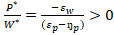
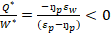
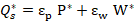
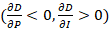
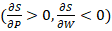
Where ƞp, ƞI, Ɛp and Ɛw denote price elasticity of demand, income elasticity, price elasticity of supply, and wage elasticity, respectively. By solving the above equations simultaneously, results in the reduced form expression for price (P*) (and equilibrium quantity (Q*).

 

 

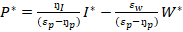
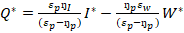
Based on the above reduced form expressions, comparative-static hypotheses have been constructed as follow:

 

=  

 

=  

Based on the comparative-static results, an increase in wage will increase price and reduce quantity. Also, an increase in income will increase the price of lettuce and the quantity of lettuce.

Econometric model and data description

In order to empirically test the derived model in equation (7) - (12), price elasticity of demand, price elasticity of supply, income elasticity of demand, and wage elasticity must be estimated.

The required demand elasticities will be estimated using the Rotterdam demand model because it is consistent with demand theory. The Rotterdam demand model is specified as below:

 

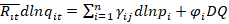
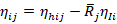
Where Ri is the budget share for good i, R̅ι equals (Rit+Rit-1)/2, pi, is the price of good i, and DQ is the Divisia volume index, which is calculated as .

In order to comply with demand theory, the Rotterdam demand model has to satisfy the following parametric restrictions:

(13.a) (adding-up)

(13.b) (homogeneity)

(13.c) (symmetry)

Unlike single equation demand estimation, the Rotterdam demand model consists of system of demand equations that allow the researcher to impose or test theoretical restrictions such as adding-up and symmetry. Moreover, the system of demand equations enables the consideration of mutual interdependence among the commodities (World Bank, 2002).

Furthermore, income elasticity and price elasticities are computed as follow:

(Income Elasticity)

(Hicksian Price Elasticity)

(Marshallian Price Elasticity)

The required supply elasticities for model calibration will be estimated using a dynamic ad-hock supply model similar to Lee and Helmberger’s (1985) model.

 

ln W, ln AP, and ln PL are the logs of labor wage, acreage planted, and lettuce price. The dynamic ad-hock model was chosen due to its simplicity and its empirical relevance to obtain the needed supply elasticities to calibrate the EDM model.

The data for the demand and supply models were obtained from the USDA database. The data used for the Rotterdam demand model is from 1960 to 2007. Moreover, the data used in the estimation of the supply model is from 1989 to 2009. Quantity and prices of lettuce in this paper is for the U.S. head lettuce data. Also, the data for wage is the crop workers’ wage rate per hour.

Results and Conclusion

The Rotterdam demand model (13) was estimated as a system of three equations consisting of lettuce, carrot, and bell pepper. The model was estimated using seemingly unrelated regression (SUR) method. The bell pepper equation was dropped to avoid singularity in the variance-covariance matrix. The estimated parameters are reported in Table 1. The R2 of the lettuce equation shows that 65 percent of the variations in the dependent variable have been explained by the independent variables. The Durbin-Watson test shows no evidence of autocorrelation. Furthermore, the results of the Shapiro-Wilk normality test indicate that the residuals are normally distributed. In addition, heteroscedasticity test was performed using White’s general test and the Breusch-Pagan test. The results of the two tests show that we fail to reject the null hypothesis of no heteroscedasticity.

The estimated income elasticity of lettuce and Marshallian own price elasticity of lettuce are reported in Table 3. The Marshallian own price elasticities were chosen for this paper because the elasticities are suitable for policy analysis. The results show that the demand for lettuce is income inelastic. Also, the results imply that lettuce is a necessity good. Moreover, the own price elasticity of lettuce has the correct sign, and the demand for lettuce is price inelastic. The estimated income elasticity (0.536) and price elasticity (-0.557) differ in magnitude compared to Hamming and Mittlehammer’s (1980) estimate. The difference is due to the fact that this paper has used a theory-based model to estimate income and price elasticity. Also, the price elasticity in this paper is Marshallian price elasticity. Moreover, this paper uses longer time-series compared

Table 1: Rotterdam model parameter estimates.

Equation	Intercept	γi1	γi2	γi3	DQ	R2	DW
Lettuce	-0.00394 (0.00279)	-0.012 (0.0153)	0.019* (0.0103)	-0.007 (0.0125)	0.536*** (0.0618)	0.65	1.72
Carrot	-0.002 (0.0023)		-0.015 (0.0107)	-0.004 (0.009)	0.395*** (0.0503)	0.60	1.87

Note: 1: Lettuce; 2: Carrot; 3: Bell pepper; standard errors in parenthesis; ***, **, * denote significance level at the one, five and ten percent level.

to Hamming and Mittlehammer’s (1980) paper, which covered the period from 1954 to 1977.

The dynamic supply model (17) was estimated with unconditional least square method with AR (2) process. In PLit-1 and In APit-1 were normalized using lettuce producer price index. The estimated parameters of the dynamic supply model are reported in Table 2. The Durbin-Watson and Godfrey’s Serial Correlation test fail to reject the null hypothesis of no autocorrelation. The Jarque-Bera normality test shows that the residuals of the dynamic supply model are normally distributed. Furthermore, the Lagrange multiplier (LM) test shows no evidence of heteroscedasticity. The estimated own price elasticity of supply is positive and inelastic. Generally, inelastic supply is common phenomena in agricultural products due to production lags and perishability. In addition, the wage elasticity is negative as expected. The partial elasticity of wage shows that a one percent increase in wage reduces lettuce supply by 0.53 percent.

Table 2: Parameter estimates for the supply model.

Variable	Estimate
Intercept	14.348***(0.2712)	R2	0.92
In APit-1	-0.275***	DW	2.12
In PLit-1	0.210***(0.0527)	Jarque-Bera normality test	0.7775
In W	-0.526***(0.0644)

 

Table 4 shows the total elasticities or reduced form elasticities for the exogenous variables, wage and income. Hypotheses (10) and (12) indicate that an increase in income increases the equilibrium price and equilibrium quantity of lettuce. Moreover, hypotheses (9) and (11) show that an increase in wage increases equilibrium price of lettuce and reduces equilibrium quantity of lettuce. Based on the results of these elasticities, the null hypotheses as specified in equations (9)-(12) are accepted. As a result, an increase in wage will increase lettuce price and decrease lettuce quantity. The results show that a one percent increase in wage decreases quantity by 0.38 percent. A one percent increase in wage increases price by 0.70 percent. Moreover, an increase in income will increase price and quantity of lettuce by 0.69 percent and 0.15 percent, respectively. In order to measure the impact of both wage and income on P* and Q* as specified in equation (7) and (8), we need to know the percentage change in wage and income. The crop worker per hour wage rate in the U.S. changed from $5.12 in 1989 to $10.07 in 2010. Thus, the percentage change in wage is 96.68 percent. The aggregate annual percentage change in wage is 68 percent, and the average annual percentage change in wage is 3.44 percent. The average annual percentage change in the U.S. per capita income from 1960 to 2007 is 6.10 percent. Table 5 shows that if income increased by 6.10 percent and wage increased by 3.44 percent; one would expect the equilibrium price of lettuce to increase by 0.522 percent and the equilibrium quantity of lettuce to decrease by 0.253 percent.

Table 3: Estimated supply and demand elasticities.

Elasticity	Estimates
ȠI	0.536*** (0.0618)
ȠP	-0.557*** (0.0624)
εP	0.210*** (0.0527)
εw	-0.526*** (0.0644)

 

Table 4: Total elasticities of wage and income.

Expression	Results	Decision
P*/ W*	0.700	Fail to Reject H0
P*/ I*	0.692	Fail to Reject H0
Q*/ W*	-0.380	Fail to Reject H0
Q*/ I*	0.145	Fail to Reject H0

 

Table 5: Combined effect of wage and income on P* and Q*.

Term	Percentage Change
P*	0.522
Q*	-0.253

 

Welfare analysis

Welfare effect is measured by the change in consumer surplus, producer surplus, and total surplus. The paper is concerned in this section with measuring the welfare effect of wage and income increase that occurred over the time frame of this study. Thus, the below formulas are used to measure the welfare effect of wage and income increase in the U.S. lettuce market (Wholgenenant, 1993; 1999; Kinnucan and Cai 2011; Sisman, 2017):

(18)

(19)

Where; the value in initial equilibrium is denoted by P0Q0, Vs is the vertical shift in the supply curve resulting from wage increase. As appeared on equations (18) and (19), we would expect the increase in wage and income to decrease producer welfare and consumer welfare. The total U.S. lettuce sales in 1992 as reported by Sexton and Zhang (1996) reached 800 million. However, the average value of lettuce during the observations of this paper differs from 800 million. Indeed, it reached 692 million. Thus, this value will be used as the initial equilibrium value. Furthermore, Vs in this paper is measured as

 

The welfare effect was measured assuming a 3.44 percent increase in wage and 6.10 percent increase in income. These values were selected since they represent the average annual percentage change in wage and income, respectively. The welfare results in Table 6 are consistent with equations’ (18) and (19) predictions. The increase in wage decreases producer surplus, consumer surplus, and consequently total surplus. However, the magnitude of the reduction in producer surplus is larger than consumer surplus.

Table 6: Welfare effect of wage and income increase.

Change in Surplus	Welfare Change
∆ PS	-728040
∆ CS	-315365
∆ TS	-1043405

* Values are in 1000 USD

Due to the fact that wage of labor involved in agricultural production in the U.S. has drastically increased, the paper is concerned with investigating the impact of wage increase on the US lettuce market. The paper has developed an Equilibrium Displacement Model to study the impact of wage and income increase on lettuce price and quantity. The comparative-static hypotheses of the paper show that an increase in wage increases price and reduces quantity. In order to calibrate the EDM model, the paper estimated lettuce demand using the Rotterdam demand model and lettuce supply using dynamic ad-hock model. The results show that the demand for lettuce is price and income inelastic. Also, the supply of lettuce is price inelastic, which is consistent with the notion that the supply of agricultural product is price inelastic due to perishability and biological factors. Also, the partial elasticity of wage shows that wage has a negative impact on lettuce supply. In fact, a one percent increase in wage reduces lettuce supply by 0.526 percent. In addition, the results of total elasticities show that an increase in income increases price and quantity of lettuce. Furthermore, the total elasticities show that an increase in wage increases lettuce price and reduces lettuce quantity. Consequently, we fail to reject the null hypotheses that were derived using comparative-static derivatives since the increase in wage increases lettuce price and reduces quantity. Finally, the paper concludes by examining the welfare effect of wage and income increase. The results show that producer surplus and consumer surplus will decrease as a result of wage and income changes. However, the magnitude of the decrease in producer surplus is larger than the decrease in consumer surplus.

References

Agricultural Marketing Resource Centre. Available at: http://www.agmrc.org/commodities__products/vegetables/lettuce-profile/ (Accessed February, 27, 2018).

Bank, W. 2002. A users guide to poverty and social impact analysis. Poverty Reduction group (PRMPR) and Social Development (SDV), Work in Progress Draft for Comment April, 19.

Bohall, R.W. 1972. Pricing performance in marketing fresh winter lettuce. Washington DC: U.S. Department of Agriculture, ERS Mark. Res. Rep. No. 956, May 1972.

Carter, C.A., D.L. Hueth, J.W. Mamer and A. Schmitz. 1981. Labor strikes and the price of lettuce. West. J. Agric. Econ. pp.1-14.

Calvin, L. and P. Martin. 2010. Labor-Intensive US Fruit and Vegetable Industry Competes in a Global Marketa. Amber Waves. 8(4): pp. 25.

Glaser, L.K., G.D. Thompson and C.R. Handy. 2001. Recent changes in marketing and trade practices in the US lettuce and fresh-cut vegetable industries. US Department of Agriculture, Economic Research Service, Agric. Inf. Bull. No. 767.

Hammig, M.D. and R.C. Mittelhammer. 1980. An imperfectly competitive market model of the US lettuce industry. West. J. Agric. Econ. pp.1-12.

Kinnucan, H.W. and H. Cai. 2011. A benefit-cost analysis of US agricultural trade promotion. Am. J. Agric. Econ. 93(1): pp.194-208. https://doi.org/10.1093/ajae/aaq115

Lee, D.R. and P.G. Helmberger. 1985. Estimating supply response in the presence of farm programs. Am. J. Agric. Econ. 67(2): pp.193-203. https://doi.org/10.2307/1240670

Muth, R.F. 1964. The derived demand curve for a productive factor and the industry supply curve. Oxf. Econ. Pap. 16(2): pp.221-234. https://doi.org/10.1093/oxfordjournals.oep.a040951

Preston, J. 2007. Short on labor, farmers in US shift to Mexico. New York Times.

Sexton, R.J. and M. Zhang. 1996. A model of price determination for fresh produce with application to California iceberg lettuce. Am. J. Agric. Econ. 78(4): pp. 924-934. https://doi.org/10.2307/1243849

Schwartzman, K.C. 2008. Lettuce, segmented labor markets and the immigration discourse. J. Black Stud. 39(1): pp.129-156. https://doi.org/10.1177/0021934706297009

Şişman, M.Y. 2017. An economics welfare analysis of agricultural subsidies and inventory holdings: An application to the hazelnut industry. Int. J. Food Agric. Econ. 5(4): pp.63-79.

Weil, R.J., E.M. Silva, J. Hendrickson and P.D. Mitchell. 2017. Time and technique studies for assessing labor productivity on diversified organic vegetable farms. J. Agric. Food Sys. Community Dev. 7(4): pp.129-148.

Welbaum, G.E. 2015. Veg. prod. Pract. CABI.

Wohlgenant, M.K. 1993. Distribution of gains from research and promotion in multi-stage production systems: The case of the US beef and pork industries. Am. J. Agric. Econ. 75(3): pp. 642-651. https://doi.org/10.2307/1243571

Wohlgenant, M.K. 1999. Distribution of gains from research and promotion in multistage production systems: reply. Am. J. Agric. Econ. 81(3): pp. 598-600. https://doi.org/10.2307/1244019

Wohlgenant, M.K. 2011. Consumer demand and welfare in equilibrium displacement models. Oxf. handbook Econ. Food Consumption policy. pp.0-44. https://doi.org/10.1093/oxfordhb/9780199569441.013.0012