Research Article

Spectral Analysis of Temperature and Rainfall Trends using Hybrid Nonparametric-Wavelet Transform Method

Khurram Sheraz* and Taj Ali Khan

Department of Agricultural Engineering, Faculty of Civil, Agricultural and Mining Engineering, University of Engineering and Technology Peshawar, Pakistan.

Received | November 01, 2021; Accepted | February 05, 2022; Published | August 29, 2022

*Correspondence | Khurram Sheraz, Department of Agricultural Engineering, Faculty of Civil, Agriculture and Mining Engineering, University of Engineering and Technology Peshawar, Pakistan; Email: [email protected]

Citation | Sheraz, K. and T.A. Khan. 2022. Spectral analysis of temperature and rainfall trends using hybrid nonparametric-wavelet transform method. Sarhad Journal of Agriculture, 38(3): 1105-1123.

DOI | https://dx.doi.org/10.17582/journal.sja/2022/38.3.1105.1123

Keywords | Discrete wavelet transform, Mann-kendall test, Periodicities, Rainfall, Temperature

Copyright: 2022 by the authors. Licensee ResearchersLinks Ltd, England, UK.

This article is an open access article distributed under the terms and conditions of the Creative Commons Attribution (CC BY) license (https://creativecommons.org/licenses/by/4.0/).

Introduction

Our planet has been significantly warmed by the greenhouse gas emissions caused by human interventions leading towards unprecedented and irreversible climatic changes. These changes are causing our terrestrial environment to transform and evolve continuously. According to (Masson-Delmotte et al., 2021), it is evident that human interventions have caused warming of the atmosphere, land, and ocean. Different approaches have been used to project hydrological parameters like snow/glacier melt and precipitation which have indicated probable increase in the flow at the basin scale up to the mid of the current century. Kundeti et al. (2022) made use of the high resolution hydrological data taken from the Coupled Model Intercomparison Project Phase 6 (CMIP6) of two Shared Socioeconomic Pathways (SSP2-4.5 and SSP5-8.5) that was statistically downscaled and corrected for biasness. Their analysis on mean precipitation and temperature changes and their extreme values over the Indus basin showed a likely increase of 40% (June-September) for temperature and 25% (December-February) for precipitation by the end of this century.

Future temperature projections show that warming may continue over the basin. Ali et al. (2015) projected river flow using data generated by Conformal-Cubic Atmospheric Model, Regional Climate Model and RCP 4.5 and RCP 8.5. They found high uncertainty in the projected future runoff for the lower and upper Indus basin (UIB) due to high spread in the winter and summer precipitation projections. A non-uniform change was observed in the projected precipitation, an upward change for the upper parts and a downward change for the lower parts of the basin. The model projections has shown an increase in the flow of UIB due to a combined effect of warming resulting in increased snow/glacier melt and increase in precipitation during summer and winter. These changes are detrimental, and therefore, the reliable characterization of global climatic changes is quite difficult due to the presence of inter-annual, multidecadal, or even longer variability in the natural climate due to anthropogenic activities (Kolokytha et al., 2017). A proper understanding of the spatio-temporal distribution and the changing patterns of temperature and precipitation is required for an effective planning and management of the water resources.

Climate change has become a menace to the economic, social, and environmental facets (Lee et al., 2015). The components of the hydrologic cycle, both in quality and quantity, are affected by the climatic variability (Pandey et al., 2017a). The hydrological setup of Pakistan is also affected by the adverse effects of climate change, and it has become a climate change “hotspot” (Kilroy, 2015). According to German Watch Report: Global Climate Risk Index 2021 (Eckstein et al., 2021), Pakistan ranks at 8th position among the most adversely affected countries having a CRI score of 29.0. According to the data collected from 2000-2019, Pakistan has faced 03% deaths per 100,000 population. The catastrophes induced by climate change have given a $3.8 billion worth of economic loss. During the recent decade, Pakistan has experienced the most terrible droughts, storms, and floods in its history (Hussain and Mumtaz, 2014). It is estimated that 126 heat waves have struct Pakistan from 1997 to 2015 i.e. about seven per year with an increasing trend (Nasim et al., 2018). More than 1200 lives lost due to the heat wave of June 2015 in Karachi (Chaudhry et al., 2015). Forty percent of Pakistan’s population is vulnerable to disasters like storms and droughts associated to the change in rainfall patterns (McElhinney, 2011).

The Indus River basin’s water availability is highly variable as the melting of its water contributing glaciers is unpredictable and the future precipitation regime is also uncertain (Bolch, 2017). Pakistan’s economy is agriculture-based and dependent on a huge irrigation system comprised of diversions, barrages and channels, mostly fed by the UIB. The livelihood of a huge population at the downstream of UIB depends on its inflow (Khan et al., 2015). Therefore, the irrigated agriculture, economy, infrastructure, human- and wildlife, all will be highly affected by any changes in the demand or supply of the UIB in future (Qin et al., 2013). Projections of future glacier change in the region have been done at regional scale. The melting of the glaciers and snow in the Karakoram, Himalaya, and Hindu Kush mountains provides more than 50% of the inflow to UIB. The increase in temperature due to the climate change will also increase the snow melting rates in the near future affecting the timing and magnitude of the generated flows (Soncini et al., 2015; Lutz et al., 2016). The mean streamflow, occurrence of the extreme events and their magnitudes, especially during the rainy seasons, will be increased (Wijngaard et al., 2017). Thus, it is very important to analyze the shifts in the meteorological indices so that better planning and adaptation could be done for the unavoidable circumstances as the lives of people depend on these precious water resources (Khan and Adams, 2019).

Data are a central part of studies that attempt to detect trends and changes in meteorological processes. It is very important to have adequate and reliable information pertaining to a watershed including data of hydrological and meteorological indices for an effective and sustainable management of the water resources (Horne, 2015). Detection of trends and analysis of past climatic data is usually done to assess the changes in climate (Adamowski et al., 2010). Many studies have been conducted on analyzing the climatic variables and detecting trends by using different techniques (Khattak et al., 2011; Mondal et al., 2015; Chandniha et al., 2017; Ahmad et al., 2018). Different parametric/non-parametric methods and graphical approaches have been used to analyze climatic trends in these studies. Ahmad et al. (2018) used an innovative trend analysis (ITA) method, Mann-Kendall (MK), and Sen’s slope estimator tests to study the annual and seasonal precipitation variability for low and high precipitation at twenty sites across the upper Indus River Basin (UIB). They detected positive trends for heavy precipitation with magnitude greater than 10% at thirteen stations during winter season and at eight stations during the summer season. The majority of the stations with significant trends were in the UIB’s north-east and north-west regions, implying that flooding in the northern regions would intensify, while flooding in the southern regions will probably decrease. They also found that extended drought occurrences are more likely to occur during the winter and spring seasons. Khattak et al. (2011) examined trends in three hydrometeorological parameters; temperature, precipitation, and streamflow for a period of 1967-2005 in UIB in Pakistan. They detected an inconsistent pattern of precipitation variability from the stations situated in the UIB’s southern region. Strong trends were detected in both indices. Significant warming trend (p < 0.10) was found in the max. temperature of winter season. Their results are strong evidence of the warming of UIB during winter and cooling of summer seasons during the study period. The different methods have been reviewed by (Sonali and Kumar, 2013).

The stationarity in the climatic indices has been commonly assumed used in the above methods. However, this assumption has been comprised due to anthropogenic activities (Milly et al., 2008). The probability distribution functions established and associated with hydroclimatic variables of a basin are affected by changes in the mean values caused by anthropogenic sources. There are nonuniform and non-monotonic changes in the climate that makes the detection of trends complicated, especially in a non-stationary environment (Franzke, 2010). Since hydrological processes may be affected by factors such as weather, vegetation cover, infiltration, and evapotranspiration, they contain stochastic constituents, and multi-time scale and nonlinear properties (Wang and Ding, 2003).

While analyzing trends in hydroclimatic time series, not only is it important to check for whether the direction of trends is positive or negative, but also how these changes fluctuate within different time-scales (i.e., intra- and inter-annual, and decadal events). Hussain et al. (2021) conducted research on the monthly minimum and maximum temperatures and precipitation data ranging from 1955-2016 for nine meteorological stations in the UIB of Pakistan by employing Mann-Kendall tests combined with continuous and cross wavelet transform to analyze the spatiotemporal variability of temperature and precipitation. Their results showed significant warming of winter temperatures and cooling of summer temperatures. The precipitation exhibited increasing trends in annual and seasonal time series although no significant change was found in the total precipitation of UIB during 1960-2012. Wavelet analysis illustrated that periodicities were usually constant over short time scales and discontinuous over longer time scales. A mathematical methodology frequently used to detect oscillatory signals is the Fourier Transform (FT), which uses sine and cosine basis functions. The FT has some major drawbacks. Since this method uses single-window analysis, it is unable to detect the properties of signals that are much shorter or longer than the size of the window. Furthermore, the sinusoids used in FT are only localized in the frequency domain and not in time domain. Therefore, FT only provides time-averaged results and extracts details from the signal frequency, but loses its time-based information (Nalley et al., 2012). The wavelet transform (WT) considers such issues by performing decomposition of a 1-D signal into 2-D time-amplitude-frequency information that renders it more effective for analyzing non-stationary time series (Karthikeyan and Kumar, 2013). In WT, variable size windows are employed to decompose a time series i.e., narrow windows (at lower scales) are used to analyze large periodicities or high-frequency components while wide windows (at higher scales) are used to analyze low-frequency components. Moreover, discontinuities, change points and trends are also demonstrated by the WT analysis. Results obtained from the trend analysis of different periodic components constituted by the WT can be

 

Table 1: Key features of the selected meteorological stations.

S. No.	Name of Station	Period of Record		Latitude (oN)	Longitude (oE)	Elevation (m) (a.m.s.l.)
		Temperature	Rainfall
1	Cherat (Nowshera)	1960-2006	1961-2010	33o 49′	71o 33′	1301
2	Chitral	1964-2003	1964-2010	35o 51′	71o 50′	1498
3	D.I. Khan	1960-2003	1960-2010	31o 49′	70o 56′	173
4	Dir	1968-2010	1968-2010	35o 12′	71o 51′	1369
5	Kakul (Abbottabad)	1960-2010	1960-2010	34o 11′	73o 15′	1308
6	Kohat	1961-2010	1961-2010	33o 31′	71o 27′	600
7	Parachinar (Kurram)	1960-2003	1960-2009	33o 52′	70o 05′	1725
8	Peshawar	1960-2006	1960-2015	34o 01′	71o 34′	359
9	Saidu Sharif (Swat)	1974-2010	1980-2010	34o 44′	72o 21′	961

 

 

utilized to identify the periodicities dominating and characterizing the trends (Rashid et al., 2015).

Materials and Methods

Study area and data

The study sites include the nine meteorological stations located in the upper Indus River basin as num bered from 1 to 9 in Figure 1 and detail given in Table 1, referred to as upper Indus basin (UIB), that spreads from northeast Afghanistan to Tibetan Plateau, and Khyber Pakhtunkhwa province of Pakistan. The UIB exists between 32.48o-37.07oN and 67.33o-81.83oE covering about 289,000 km2 of area. The Indus basin is among the largest basins of the world. The transboundary Indus River basin covers 112 MHa of area divided among Afghanistan (6%), China (8%), India (39%), and Pakistan (47%). It encompasses 65% Pakistan’s territory (about 52 million Ha), covering full areas of Khyber Pakhtunkhwa and Punjab and large parts of Balochistan and Sindh (Frenken, 2013).

Data of the two important meteorological variables; mean air temperatures (oC) and total rainfall (mm) from Pakistan Meteorological Department (PMD) for nine stations in UIB was acquired for the current research study (Figure 1). The criteria used for selecting stations was completeness and availability of the required data of at least forty years. The various steps involved in the data analyses are depicted in the flowchart of Figure 2.

The data was categorized in monthly, seasonal, seasonally-based and annual time series for conducting different analyses. In the monthly data, observed values from January-December were included. The seasonal data included four seasons: (i) winter including months from December-February; (ii) Spring: March-May; (iii) Summer: June-August; and (iv) Autumn: September-November. Each season was analyzed separately. The seasonally-based data analysis used the mean/total value of each season every year. The effects of the shorter time scales (e.g. intra-annual and inter-annual periodicities) on the observed trends were investigated by using the monthly data. The effects of semi-annual and annual seasonality on the trends were investigated using seasonally-based time series. The annual time-series were investigated for longer time scale events like multi-year and decadal.

Homogeneity of data

Use of unreliable climatic data may produce wrong conclusions on the climate conditions. It is a difficult task while dealing with the meteorological datasets as

 

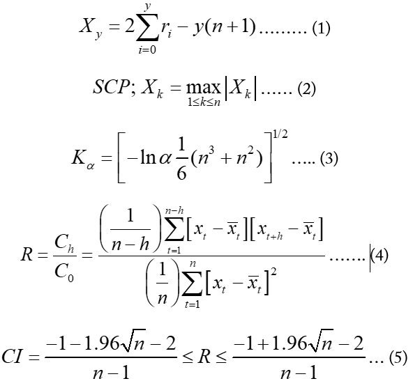
there may be changes in the observational methods and measurement procedures, environmental characteristics and structures, and station locations making the data inhomogeneous. Therefore, data quality control and homogeneity tests are conducted to minimize the error. The Pettitt’s test (Pettitt, 1979) was selected for this study to check the homogeneity of the monthly time series since it is a non-parametric, change point detection test and does not require any assumption regarding the statistical distribution of the data. This test is based on the rank, ri of the ith observation of the time series Yi and ignores the normality of the series. (Equation 1).

Where;

Xy is the Mann-Whitney test statistic, n is the number of observations and y is the number of years that takes values 1, 2, …, n. The break point occurs in year k when the estimated value Xk determined using the following Statistical Change Point (SCP) test exceeds the critical value Kα. (Equation 2).

The values obtained from eq. (2) values were compared with the following critical value Kα at significance level α = 5%. (Equation 3).

Autocorrelation

Autocorrelation is an important index to determine randomness and cyclic pattern in the data. Randomness of data is required by most traditional statistical tests. It directly affects the validity of the conclusions derived from the tests. Autocorrelation Functions are used to determine randomness or similarity between original data values and those of the same series but lagged at varying time intervals. Autocorrelations should be close to zero for all time-lags in order for the data to be random. If non-random, then one or more of the autocorrelations will be significantly non-zero (Box et al., 2015).

Different types of MK tests were applied based on the existence of autocorrelation and seasonality in the time series. The data was checked for presence of autocorrelation to know whether it is random or not. If the data is not random then it increases the chance to produce type-1 error due to underestimation of the variance (Hamed and Rao, 1998; Yue et al., 2002b). Generally, the autocorrelation is more probable in the monthly and seasonal time series. The Autocorrelation Function (ACF) at lag-h was determined as follows (Mohsin and Gough, 2010): (Equation 4).

Where;

R is the ACF at lag-h (h = No. of lags), Ch is the autocovariance function and C0 is the variance function. The value of R was checked against the following bound at 5% significance level. (Equation 5).

The ACFs were computed at lag-1 (and correlograms (Figure 5) showing the relationship between ACFs at various lags and the corresponding lags were plotted using MATLAB. An autocorrelation plot depicts either a positive or negative correlation in the data or shows that a time series is non-random. ACF’s value ranges from -1 to 1 showing negative and positive autocorrelation, respectively (-1 and 1 being perfect autocorrelations). ACF values falling outside the 95% bound specify statistically significant values (lag-0 is always 1 showing 100% autocorrelation as the value is tested against itself). An autocorrelation with lag-1 (taken on x-axis) represents the correlation between the successive observations of a time series i.e., the values and the corresponding values that were observed one time intervals earlier (Anderson, 2015). The null hypothesis of independence of data was accepted if the ACF falls within the above interval in the correlograms, and the time series is considered random.

Seasonality

A time series has seasonality if different distributions exist at different times in a year (Hirsch and Slack, 1984). The oscillations or seasonality in the data were visualized by correlograms of temperature and rainfall series. The monthly and seasonal time series and detail periodic components are anticipated more to have seasonality patterns (Choi et al., 2011) and were examined for the existence of seasonality patterns through correlograms.

Mann-Kendall Trend Test

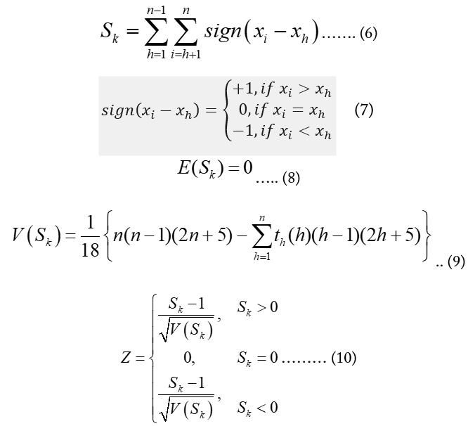
The original Mann-Kendal test proposed by (Mann, 1945) and (Kendall, 1975) was applied to the time series without significant autocorrelation in the data. It is a rank correlation test for two datasets between the rank of the values and the ordered values in the dataset. The null hypothesis of the test considers the dataset (xh, h = 1, 2, 3, . . ., n) independent and identically distributed (Yue et al., 2002b). The MK test statistic (Kendall’s tau), is given by: (Equation 6).

Where;

xi represents the ordered data values, and n denotes the length of observations; the sign test as given by (Yue et al., 2002a) is: (Equation 7).

The statistic Sk is normally distributed (approx.) having zero mean for n ≥ 10. The mean and variance of Sk can be determined by the following equations: (Equation 8 and 9).

Where;

th denotes the number of ties to the extent h. The standardized test statistic for the MK test can be determined by using the relationship given below: (Equation 10).

Positive values of Z obtained from eq. (10) represents an upward (increasing or positive) and vice versa. The Z values were compared with the standard normal variate at 5% significance level (Hamed and Rao, 1998).

Modified Mann-Kendall Trend Test

The original MK trend test is valid for a time series that does not demonstrate autocorrelation (Mohsin and Gough, 2010). For time series having significant autocorrelation, the following formula was developed by (Hamed and Rao, 1998) developed a formula based on an empirical approximation/experiment, which modifies the variance of Sk of the original MK test. (Equation 11).

Where;

n*e denotes the effective number of samples required to account for the autocorrelation in the time series. n/(n*e) is the correction factor associated with the autocorrelation of the data. Empirically, n/(n*e) is expressed as (Equation 12).

ρe(f) indicates the significant autocorrelation function between the ranks of the data, determined by using the inverse of the equation (13) as given by (Kendall, 1975). This converts the rank autocorrelation into the normalized data autocorrelation because for the evaluation of the variance S, the estimate of the normalized autocorrelation structure is required for data X whose distribution may not be normal or rather arbitrary (Hamed and Rao, 1998): (Equation 13).

Seasonal Mann-Kendall Trend Test

The seasonal Kendall test proposed by Hirsch and Slack (1984) is suitable for use with data that exhibit seasonality pattern and autocorrelation (Kundzewicz and Robson, 2004). Using a Monte Carlo experiment, Hirsch and Slack (1984) demonstrated that the seasonal Kendall test can be used with data exhibiting autocorrelation. Let the matrix x is given as; (Equation 14).

Matrix x represents a dataset containing observations taken over “v” seasons for “u” years (without any missing values or ties). Another matrix “r”, represents the ranks of the data in matrix “x” (Hirsch and Slack, 1984). (Equation 15).

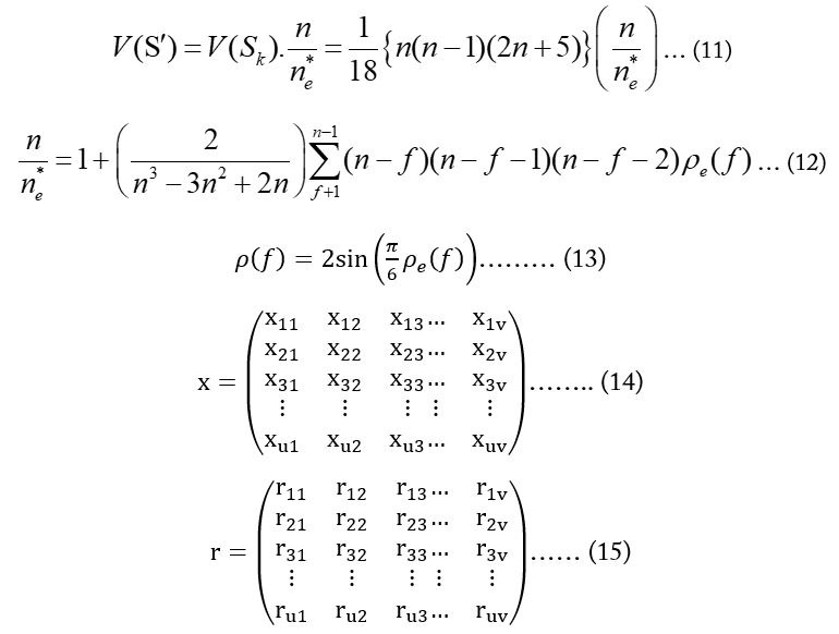
As the observations within each season are ranked among themselves, the ranks (riz) are computed using the following equation, and where each column in matrix “r” is a “permutation of (1, 2, …, n)”: (Equation 16).

The test statistics “Sz” is determined (for each season) using: (Equation 17).

The test statistics Ss for the seasonal Kendall is determined by: (Equation 18).

with a variance of (Equation 19).

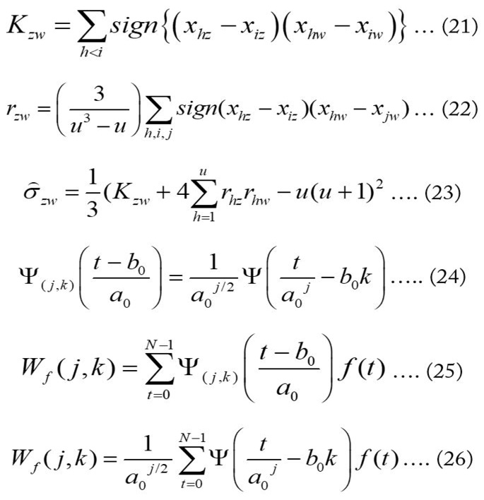
σ2z is the variance of “Sz” and represents the covariance of “Sz” and “Sw”. The estimator of the covariance is σzw (Dietz and Killeen, 1981): (Equation 20).

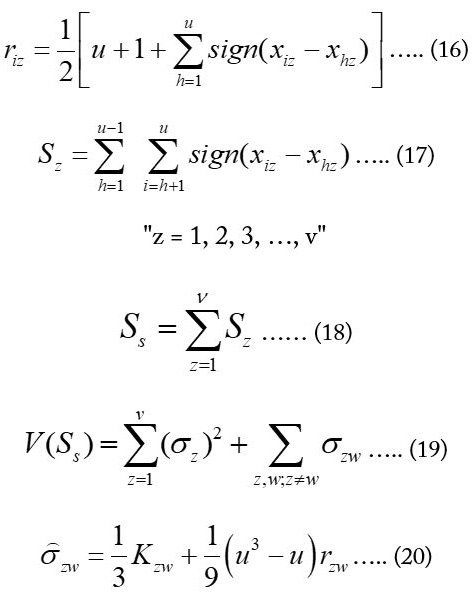
Where;

Kzw is represented by: (Equation 21).

and is calculated using: (Equation 22).

If there are no missing observations as well as no tied values, rzw is equal to the Spearman’s coefficient of correlation for z and w seasons. If we adopt the estimates of σzw to compute the variance then there is no need to assume the data as independent. The estimator of the covariance with no missing values becomes (Hirsch and Slack, 1984): (Equation 23).

Spectral Analysis using Discrete Wavelet Transform (DWT)

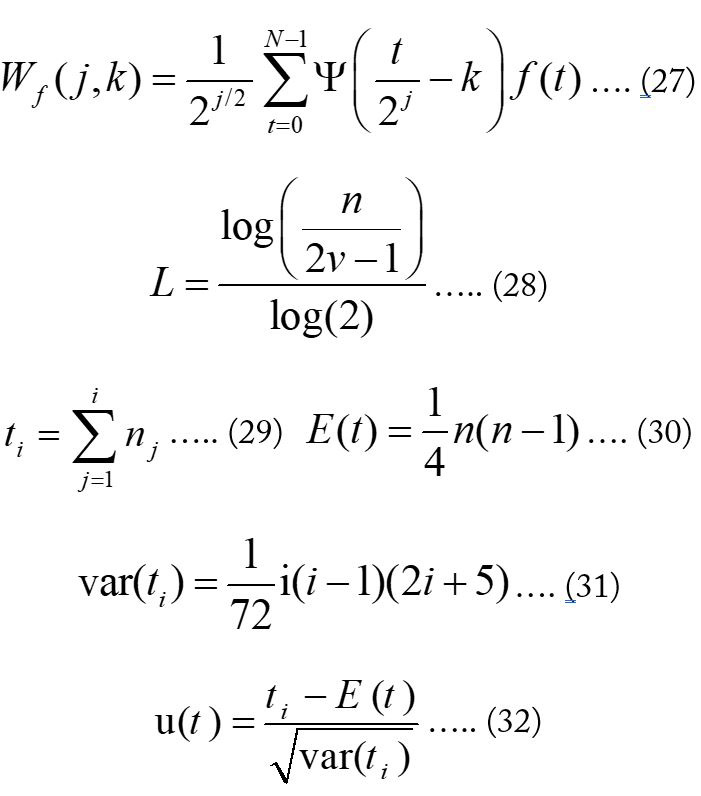
Wavelet analysis’ main goal is to get detailed information about the localized and transient phenomena happening in the signal at various temporal scales (Labat, 2008). There are two types of wavelet analyses viz. discrete and continuous wavelet analysis. The continuous wavelet analysis is used to get information about the scale (frequency) of a signal and the way the components vary in time. While the discrete wavelet analysis is employed to decompose a signal into sub-signals by using a proper wavelet and decomposition level. Most of the meteorological elements are observed or measured at a discrete interval and assuming the non-linear trends occurring gradually and lying in the low-frequency (deterministic) modes of the time series, these were converted into high- and low frequency components by employing the discrete wavelet transform. The discrete wavelet transform of a finite series f(t) at discrete integer time step by using a suitable mother wavelet ψ(t) and decomposition level j is given by (Partal and Küçük, 2006): (Equation 24, 25 and 26).

Integers j and k represent the scaling (dilation) and translation (time position) factors, respectively, a0 is the specified dilation step; whose value is constant and greater than 1, b0 is the location variable (b0 > 0), Ψ represents the mother wavelet while Wf (j, k) denotes the discrete wavelet coefficient under scale j and translation k. Practically, the orthogonal DWT (i.e. dyadic) in eq. (26) is utilized by putting: a0= 2 and b0 = 1 (Daubechies, 1992): (Equation 27).

The dyadic (integer power of 2; 2n) DWT decomposes a series into a series of “Approximation” and “Detail” coefficient sets (sub-signals) under each level which reveal the variation of the original signal at different scales and locations. These sub-signals may represent deterministic components and noise and summing to the original series. The maximum Decomposition Level L in dyadic DWT for each time-series was calculated as (Pandey et al., 2017b): (Equation 28).

L: Maximum decomposition level; N: No. of records in the data; v: No. of vanishing moments of a Daubechies wavelet (= half the filter length).

Daubechies (db5) Mother Wavelet having a 10-point filter length was chosen for decomposition of the signal (i.e. observed data) due to their orthogonality, compact support, and ease of use (Vonesch et al., 2007) indicating that the wavelets possess non-zero basis functions over a finite interval as well as translational orthonormality properties and full scaling.

Sequential Mann-Kendall Analysis

The Sequential MK Rank analysis identifies the most influencing periodic components that characterize the observed trends (Sneyers, 1990). It creates a progressive series 𝑢(𝑡) and a backward series u′(𝑡). The test Statistic ti is determined as (Equation 29).

The mean 𝐸(𝑡) and variance var(𝑡𝑖) for ti are determined as: (Equation 30 and 31).

The progressive value is determined as; (Equation 32).

The sequential Mann-Kendall values of each of the detail components plus approximation were plotted against the sequential Mann-Kendall values of the observed data. The bounds in the plots show the confidence limits of the standard normal score “Z” values at α = 5% in the sequential MK plots. Therefore, these limits correspond to ±1.96. A significant trend is indicated at α = 5% if the progressive MK value goes beyond the upper or lower C.I.; a significant positive trend if the upper limit crossed and vice versa.

 

Table 2: Results of the petitt homogeneity test for mean monthly temperature series.

Meteorological Station	p Value	Change Point at Year
Abbottabad	0.255	1972
Chitral	0.919	1998
D. I. Khan	0.994	1998
Dir	0.800	1998
Kohat	0.790	1984
Nowshera	0.174	1974
Parachinar	0.134	1991
Peshawar	0.822	1984
Swat	0.897	1999

 

Table 3: Results of the pettitt homogeneity test for total monthly rainfall series.

Meteorological Station	p Value	Change Point at Year
Abbottabad	0.177	1971
Chitral	0.043*↑	1985
D. I. Khan	0.125	1989
Dir	0.166	1979
Kohat	0.250	1997
Nowshera	0.651	1978
Parachinar	0.003*↓	1966
Peshawar	0.001*↑	1989
Swat	0.494	1992

* significant shift (↑ upward or ↓ downward) at 5% significance level

 

Most Influential Periodic Components Affecting Trends

The periodic components (periodicities) that were dominant in characterizing the trends over the study area were found firstly by comparing the MK-Z values of the observed data with their respective detail plus approximation components. Secondly, by plotting the sequential MK values of the detail plus approximation components along with sequential MK values of the observed series and looking for the similarity between the progressive trends of the two plots. Nalley et al. (2012) found that the results obtained after combining the detail components were not always conclusive. Hence, individual detail components (plus last approximation) were chosen for the sequential MK analysis. Also, since the approximation periodic components are representative of the large-scale variability (i.e. trends) (Kallache et al., 2005), it makes sense to add them to the detail periodicities prior to applying the appropriate MK test. This provided clearer information about the most dominant periodicities affecting the trends.

Results and Discussions

Homogeneity of Data

Homogeneity of the data used in this study was checked by applying the two-tailed Pettitt’s test at α = 5%. The two-tailed Pettitt’s test p values for the mean monthly temperature and total monthly rainfall are tabulated in Table 2 and 3, respectively.

The results of the Table 2 show that the time series of the mean monthly temperatures of all stations are homogeneous at α = 5%. For total monthly rainfall, significant upward shifts in the mean values were observed at the stations Chitral (mean “mu” value increased from 33.40 mm to 42.34 mm after the year 1985) and Peshawar (mean increased from 31.72 mm to 41.13 mm after the year 1995) showing inhomogeneities and significant monotonic trend tendency in the data (Figure 3). At the station Parachinar, a significant downward shift occurred in 1966 and the mean value decreased from 117.07 mm to 61.24 mm as shown in Figure 4. The quality and quantity of observed data (e.g., absence of in situ observations, measurement errors, and space–time discontinuities) restrict reliable estimates of high-altitude precipitation climatologies and quantities in the Indus basin. Dahri et al. (2018) reported that till 1969, the non-recording Symon’s gauge was most extensively used to measure rainfall in India. Afterwards, Bureau of Indian Standards adopted the Indian standards for design and manufacture of meteorological equipment, with the Indian rain gauge (20-22-P) being the most widely used. Similarly, PMD has mostly used the non-recording rain gage model MK2 (13-15-C). Then, in 2010, PMD began using tipping bucket rain gage. WAPDA is using both automatic weighing, and standard meteorological service manual rain gages. At high altitudes, WAPDA has also installed 20 automatic data collection platforms that employ snow pillows for the measurement of both solid and liquid precipitation as water equivalent. Although no solid reason was found for inhomogeneity in the observed data of rainfall of the above stations but the changes in the measuring instruments and units reported by Dahri et al. (2018) could effectively shift the mean values for the long-term data used in this study. The inhomogeneous data was corrected using double mass analysis before further use.

 

Autocorrelation and Seasonality

The monthly temperature data of all the selected meteorological stations showed significant autocorrelation coefficients at lag-1 at 5% significance level which indicated that the observations within the time series were not random and independent. The autocorrelation analysis of the time series of seasonal and annual datasets of temperature showed that the ACFs for winter season were only significant for station Abbottabad. Similarly, ACFs for spring season were found significant only for stations Abbottabad and Parachinar. Four stations, Chitral, D.I. Khan, Peshawar and Swat did not exhibit significant autocorrelation for the summer temperature series while except stations Chitral, D.I. Khan, Dir and Swat all other showed significant autocorrelation for the autumn temperature series. For the annual temperature series, no significant autocorrelation was found for Chitral, D.I. Khan, Kohat and Swat stations.

The lag-1 ACFs for the different temperature time series used in this research study are presented in Table 4. The autocorrelation charts for all the monthly temperature series showed repeated fluctuations, and thus, strong seasonality patterns. Semiannual and annual seasonality patterns were very strongly visible in all the monthly data as high ACFs were found at every 6th lag as shown in Figure 5.

 

Each of the monthly, seasonally-based, and annual time series for total rainfall was tested for autocorrelation to determine the existence of non-random characteristics at lag-1 and to see repeated fluctuations for assessing seasonality patterns. The ACF values for the monthly, seasonally-based, and annual time series of the rainfall are given in Tables 5 and 6, respectively.

It is evident from the above Tables 5 and 6 that the autocorrelation in the monthly data is more pronounced as compared to that of the seasonally-based data for total rainfall. The seasonality patterns were also visualized and determined from the respective correlograms. Seasonality was found in all monthly and seasonally-based data. The presence of strong annual cycles was visible and evident from the high coefficients in correlograms, which were repeating at

 

Table 4: Lag-1 autocorrelation functions (ACFs) of the observed temperature time series for selected meteorological stations.

Station	Monthly	Winter	Spring	Summer	Autumn	Annual
Abbottabad	0.83* ᴪ	0.30*	0.31*	0.45*	0.39*	0.63*
Chitral	0.85* ᴪ	0.28	0.25	-0.09	0.27	0.17
D. I. Khan	0.83* ᴪ	0.08	0.13	0.19	0.12	0.15
Dir	0.84* ᴪ	0.26	0.23	0.34*	0.06	0.44*
Kohat	0.83* ᴪ	-0.10	0.18	0.38*	0.30*	0.21
Nowshera	0.81* ᴪ	0.07	0.16	0.45*	0.45*	0.50*
Parachinar	0.82* ᴪ	0.02	0.36*	0.55*	0.59*	0.51*
Peshawar	0.84* ᴪ	-0.03	0.27	0.09	0.32*	0.17*
Swat	0.84* ᴪ	0.11	0.15	-0.03	0.21	0.25

* significant serial correlation at lag-1 at 5% significance level; ᴪ presence of seasonality.

 

 

every twelfth lag for monthly time series and every fourth lag for seasonally-based time series. The influence of this yearly cycle on trends is more prominent in the seasonally-based discharge, where the 2nd level of dyadic decomposition (D2) represents the 12-month dominant periodicity.

Significance of trends in the Observed Time Series

The different versions of MK trend tests were applied considering the results of the autocorrelation and seasonality to inspect the existence of significant trends in the observed time series and the detail and approximation periodic components extracted by using the discrete wavelet transform. The original MK trend test (Mann, 1945; Kendall, 1975) was selected for those time series which neither exhibited significant autocorrelation at lag-1 nor seasonality patterns. The modified version of the MK trend test (Hamed and Rao, 1998) was used for all those time series which showed significant autocorrelation at lag-1 without seasonality patterns. The modified MK trend test (Hirsch and Slack, 1984) was applied to monthly and seasonally-based time series showing a seasonality pattern. The results of the different types of the MK tests applied on the various time series of temperature and rainfall are presented in the Tables 6 and 7, respectively.

 

Table 5: Lag-1 autocorrelation functions (ACFs) of the observed rainfall time series for selected meteorological stations.

Station	Monthly	Seasonally-Based	Annual
Abbottabad	0.18* ᴪ	-0.17* ᴪ	-0.12
Chitral	0.42* ᴪ	0.08ᴪ	0.61*
D. I. Khan	0.25* ᴪ	0.11ᴪ	0.54*
Dir	0.20* ᴪ	-0.02ᴪ	0.35*
Kohat	0.18* ᴪ	0.06ᴪ	-0.67*
Nowshera	0.16* ᴪ	0.08ᴪ	-0.12
Parachinar	0.30* ᴪ	0.19* ᴪ	0.40*
Peshawar	0.16* ᴪ	0.06ᴪ	0.15
Swat	0.21* ᴪ	-0.06ᴪ	0.60*

* significant serial correlation at lag-1 at 5% significance level; ᴪ presence of seasonality

 

Mean Air-Temperature Trends

The climatic condition of the study area was found highly diverse in terms of mean temperatures. It is evident from the MK-Z values as tabulated in the above Table 6 that mixed trends (i.e. both positive and negative) were observed for temperature data in different seasons of the selected stations. For the monthly temperature data, only stations Nowshera and Parachinar exhibited significant negative trend while only station Peshawar experienced a significant positive trend. For winter temperature series, stations Chitral, Dir, Kohat and Peshawar showed significant positive trends while stations Nowshera and Parachinar showed significant negative trends. During spring season, only Kohat and Peshawar stations experienced significant positive trends, while only stations D.I. Khan, Nowshera and Parachinar showed significant trends during summer season. For the autumn data series, only station Nowshera’s time series exhibited a significant negative trend. In the annual series, only Kohat and Peshawar stations showed increasing trends while stations Nowshera and Parachinar experiences decreasing trends.

 

Table 6: MK-Z Values of the mean temperature series.

Station	Monthly	Winter	Spring	Summer	Autumn	Annual
Abbotta- bad	-1.82	-0.37	-0.04	-1.14	-1.35	-0.96
Chitral	1.36	3.41*	1.29	-1.57	0.83	1.36
D.I. Khan	-0.17	1.02	0.33	-2.09*	-0.21	-0.25
Dir	1.54	2.45*	1.53	-0.92	-0.06	1.09
Kohat	1.48	2.20*	2.25*	0.00	0.54	1.97*
Nowshera	-4.63*	-2.13*	-1.30	-3.67*	-5.17*	-5.70*
Parachinar	-3.77*	-2.52*	-1.30	-3.87*	-1.94	-2.65*
Peshawar	2.95*	2.64*	2.99*	-1.34	1.79	2.73*
Swat	0.91	1.52	1.83	-0.63	0.04	1.46

* significant trend at α = 5%.

 

Total Rainfall Trends

The rainfall trends found in the different time series categories are given in Table 7. The temporal distribution was found highly variable during different seasons in the study area. Most of the trends were found non-significant at α = 5%. For the monthly rainfall data, positive trends were found for all selected stations (including significant trends for stations Chitral, and Peshawar only) except for stations Nowshera, Parachinar and Swat having weak negative trends. Similarly, only stations Nowshera and Parachinar showed negative trends for seasonally-based data while other experience positive trends including significant trends for stations Peshawar, D.I. Khan, and Chitral. For the annual season, only three stations Peshawar, D.I. Khan, and Chitral showed significant positive trends.

 

Table 7: MK-Z Values of the total rainfall series.

Station	Monthly	Seasonally-Based	Annual
Abbottabad	0.63	0.63	-0.11
Chitral	3.90*	6.21*	3.16*
D. I. Khan	1.94	9.17*	5.36*
Dir	0.47	0.80	0.81
Kohat	0.24	0.21	0.51
Nowshera	-0.22	-0.22	-0.17
Parachinar	-1.42	-1.34	-1.49
Peshawar	2.94*	2.87*	2.57*
Swat	-0.18	0.21	0.50

* significant trend at α = 5%.

 

 

Table 8: Dominant periodicities for various mean temperature series.

Series	Peshawar	Chitral	D. I. Khan	Abbottabad	Dir	Kohat	Nowshera	Parachinar	Swat
Monthly	2.95*	1.36	-0.17	-1.82	1.54	1.48	-4.63*	-3.77*	0.91
D3+A6	-	-0.85	-	-	-	-	-	-	0.58
D3+A7	1.16	-	-3.11*	-2.58*	0.62	-0.04	-5.99*	-4.37*	-
Winter	2.64*	3.41*	1.02	-0.37	2.45*	2.20*	-2.13*	-2.52*	1.52
D1+A3	2.99*	3.58*	0.90	-0.41	-	2.21*	-2.49*	-2.44*	1.50
D2+A3	-	-	-	-0.09	2.77*	1.65	-	-2.05*	-
Spring	2.99*	1.29	0.33	-0.04	1.53	2.25*	-1.30	-1.30	1.83
D1+A3	4.14*	-	-0.17	-0.10	1.28	2.90*	-1.98*	-1.31	2.68*
D2+A3	-	1.54	-	-	-	2.28*	-1.31	-1.40	-
Summer	-1.34	-1.57	-2.09*	-1.14	-0.92	0.00	-3.67*	-3.87*	-0.63
D1+A3	-1.80	-2.02	-2.09*	-0.92	-1.73	-0.46	-6.15*	-3.31*	-0.09
D2+A3	-	-	-	-	-	-	-	-	-0.64
Autumn	1.79	0.83	-0.21	-1.35	-0.06	0.54	-5.17*	-1.94	0.04
D1+A3	3.58*	0.99	-1.45	-1.34	-	-	-	-	0.04
D2+A3	-	-	-	-	-0.34	0.35	-6.95*	-1.91	-0.13
Annual	2.73*	1.36	-0.25	-0.96	1.09	1.97*	-5.70*	-2.65*	1.46
D1+A3	3.39*	1.90	-1.06	-	-	-	-5.76*	-	1.92
D2+A3	-	-	-	-0.60	0.94	1.64	-4.71*	-2.92*	-

 

Spectral Analysis using Discrete Wavelet Transform (DWT)

The MATLAB’s multilevel one-dimensional (1-D) wavelet decomposition function was used to perform the discrete wavelet analysis on each time series because the mean air-temperature and total rainfall were one-dimensional. The monthly and the seasonally-based time series included large number of values. Using db5 as the mother wavelet and eq. (28), all monthly temperature and rainfall time series were decomposed into seven decomposition levels (D1–D7) and one approximation level (A7) based on the data length as there were more than 512 (i.e. 29) data points that shifted the dyadic scale to next level i.e. 210 except for two stations Chitral and Swat which were decomposed into six levels (D1–D6) as their data length was less than 512. An example of the multilevel 1-D decomposition for the monthly mean temperature data of station Abbottabad is presented in Figure 6. Similarly, the seasonal time and annual series for temperature and rainfall were decomposed into three detail (D1–D3) and one approximation (A3) levels with an exception for station swat whose annual total rainfall series contain two decomposition levels. The seasonally-based time series for rainfall was decomposed into five detail (D1–D5) and one approximation (A5) components except for station Swat having four decomposition levels. Since, the wavelets were produced at dyadic (2n) scales, therefore, D1 represents the 2-unit (a unit be either a month, season or year depending upon the category of the time series) time periodicity; D2 represents the 4-unit, D3: 8-unit; D4: 16-unit; D5: 32-unit; D6: 64-unit; and D7 represents 128-unit periodicity.

Dominant Periodicities Affecting Trends

The dominant periodicities affecting the trends were determined firstly by applying the suitable versions of MK tests using XLSTAT and secondly by performing sequential MK analysis and observing the similarities between the progressive trend plots of the observed series and those of the detail plus last approximation components. It is illustrated in Figure 7 that how the most dominant periodicities affecting trends were determined graphically by visualizing similarity in the progressive trends. The sequential values are important to be analyzed because a time series may contain a mixture of positive and negative trends which may cancel each other and finally produce a non-significant trend value.

The MK analysis performed on the detail (D) and approximation (A) periodic components that were extracted from the monthly mean temperature series by DWT showed that two detail components (D5 and D6) of station Chitral having MK-Z trend

 

values -2.08 and 2.00, respectively, were found significant. But after adding the approximation components of the last decomposition level to the detail components and testing the resultant series with MK tests, most of the trend values for various stations became statistically significant. The comparison of trend values of the observed time series with those of the resultant series (detail + approximation components) as well as the results of the sequential MK analysis showed that the 8-monthly periodicities (D3) dominated the trends, as given in Table 8.

Analysis of temperature trends in winter shows that winter has experienced warming trends in most of the stations having significant positive trend values as shown in Table 6 and 8. These results agree with the results of (Khattak et al., 2011; Hussain et al., 2021). The plots of the sequential MK analysis and comparison of the trend values showed that the winter’s temperature trends of most of the stations were affected by 2-yearly (D1) periodicities except station Dir \whose dominant periodicity was D2 (4-yearly). D2 was also found the most dominant periodicity for stations Abbottabad, Kohat and Parachinar, which represents the 4-yearly cycle. For spring temperature series, only two stations Peshawar (+2.99) and Kohat (+2.25) experienced significant increase in the mean temperatures as given in Table 6. The D1+A3 i.e. 2-yearly periodicity has been found most effective and dominating the spring temperature except for station Chitral which is dominated by D2 (plus A3) representing 4-yearly cycle. Table 8 shows that the stations Kohat, Nowshera and Parachinar were also affected by the 4-yearly periodicity. The results of the MK tests showed that all stations have experienced negative trends for summer temperature including significant decreasing trends for D.I. Khan, Nowshera and Parachinar stations which showed that the summer mean temperatures have been decreased over the study period. Significant cooling of the summer season has also been reported by (Khattak et al., 2011; Hussain et al., 2021). It is evident from the sequential MK plots that D1+A3 components representing 2-yearly periodicities were in harmony with those of their respective observed time series. For station Swat, the 4-yearly cycle (D2+A3) along with D1+A3 was also affecting the summer temperature trends as evident from Table 8. The result showed that the most dominant periodicities characterizing the trends of autumn temperature were varying spatially in the study domain. It was found that the periodicity D1 (2-yearly) and D2 (4-yearly) were the most dominating periodicities. The station Swat was affected by both D1 and D2, showing more variability in the trends. The analysis of seasonal mean temperatures presented above clearly show warming over the sites as significant positive trends dominated on their negative counterparts, especially in the seasons of winter and spring as given in Table 6.

The annual mean temperature time series was investigated to achieve a detailed analysis. It was found that the addition of approximation components to the detail components increased the values of trends. Two stations, Peshawar and Kohat showed significant warming while only two stations Nowshera and Parachinar experienced significant decreasing trend values. The 2-yearly (D1) and 4-yearly (D2) periodicities were found dominant in affecting the annual temperature trends as shown in Table 8. The annual trends were found mostly consistent with monthly and seasonal trends except for station Dir whose annual trend seems to be a result of negative and positive seasonal trends.

For the monthly rainfall data, only stations Peshawar and Chitral showed significant positive trends for the observed data as given in Table 7. Similarly, only the periodic component D7 and D4 showed significant values for stations Chitral and Swat, respectively. But after adding the approximation component of the signals to their respective detail components, several MK-Z values became statistically significant. The results given in Table 9 also indicate that the detail components are affected by their approximation counterparts as the later increased their values and made them statistically significant (in most of the cases). This showed that the approximation component of the wavelet analysis contained the trends and that the trends changed slowly and gradually. The results of the MK tests and sequential MK analysis showed that for most of the stations, 8-monthly (D3+A3) and higher periodicities were influential on the trends while for stations Abbottabad, Dir, Kohat and Swat 4-monthly periodicities were also found dominant as given in Table 9.

The seasonally-based total rainfall time series was included in this study because annual cycles were identified in the monthly time series investigations. It also validated the existence of annual oscillations in the data sets as the autocorrelation function showed maximum

 

Table 9: Dominant periodicities for various total rainfall series.

Series	Peshawar	D. I. Khan	Abbottabad	Dir	Kohat	Nowshera	Parachinar	Chitral	Swat
Monthly	2.94*	3.90*	1.94	0.63	0.47	0.24	-0.22	-1.42	-0.18
D2+A7	-	-	-	-0.67	0.38	1.12	-	-	-0.51
D3+A7	5.07*	4.19*	4.06*	-	-	-	0.66	-3.50*	-
Seasonally-based	2.87*	6.21*	9.17*	0.63	0.80	0.21	-0.22	-1.34	0.21
D1+A5	0.84	5.59*	-	-	1.65	-	-1.65	-3.05*	0.12
D2+A5	-	-	6.31*	0.69	-	-0.39	-	-	-
Annual	2.57*	3.16*	5.36*	-0.11	0.81	0.51	-0.17	-1.49	0.50
D1+A3	3.23*	3.44*	3.93*	-	1.02	-	-2.72*	-	-
D2+A3	-	-	-	-2.28*	-	0.52	-	-0.77	-
D3+A3	-	-	-	-	0.86	0.51	-	-	-

 

values at every 4th lag. These oscillations did not weaken over time. Cyclic patterns were also found at higher levels of decomposition, but they got weakened with increasing number of lags. The repeated cycles observed for the lower levels of decomposition were obvious as they captured the oscillating characteristics (seasonality), and thus, filtered the stochastic components of the time series. Positive trends were detected in the original seasonally-based series except for Nowshera and Parachinar stations; three stations also experienced significant increasing trends i.e. Peshawar (+2.87), Chitral (+6.21), and D.I. Khan (+9.17) as given in Table 7. It was found that 6-monthly and 1-yearly periodicities (D1 and D2) have contributed to the trend formation in the long-term rainfall data as given in Table 9.

For annual total rainfall series, three stations: Peshawar (+2.57), Chitral (+3.16), and D.I. Khan (+5.36) experienced significant positive trend values. All other stations showed non-significant trend values for the observed data as given in Table 7. It is obvious from Table 9 that the decomposition levels of the dominant periodicities who are the major contributors in affecting the annual total rainfall are not uniform. The most common influential periodic components are D1 and D2 (plus their approximations). This indicates that 2- to 4-yearly periodic events (interannual fluctuations) have characterized the trends of annual rainfall of the selected stations. Two stations, Dir and Kohat were also found affected by 8-yearly rainfall cycles.

Conclusions and Recommendations

The current research study finds the transformation of the meteorological time series using discrete wavelet transform very effective in extracting the hidden information from the data which is otherwise not visible in the raw data. Thus, trends and the dominant periodicities are determined precisely. The findings revealed that the temperature trends were governed by the resultant of summer and winter trends. The higher-resolution data (mean monthly temperatures) were influenced by intra-annual periodicities of 8-months periods. The lower-resolution data (seasonal and annual temperatures) were highly affected by multiyear periodicities mostly ranging from 2- to 4-years. The MK analysis on seasonal data showed that the winters have experienced significant warming over the study area except for stations Nowshera and Parachinar while summers have experienced decreasing temperature trends. Rainfall trends were mostly dominated by positive trends. The monthly data was dominated by intra-annual periodicities ranging from 2-8 months. The seasonally-based and annual data were highly influenced by multiyear periodicities ranging from 2-4 years, and 2-8 years, respectively.

Acknowledgements

I am grateful to my research supervisor and members of the research evaluation committee for their technical support and guidance throughout my PhD research work. I am also very much thankful to PMD for providing the required data. The manuscript has not been published or submitted to other journals previously.

Novelty Statement

Many studies have been conducted for detecting monotonic climatic trends using conventional methods like Mann-Kendall test, Sen’s slope, and regression etc. Most of the studies were limited to assess trends in the observed data only without exploring the root causes for their development. However, for efficient and effective management of water resources, time periodicities which are hidden in the raw data need to be detected to determine the time scales responsible for the development of trends and to analyze their long-term behavior. In this study, the historical climatic data of the selected stations have been used to assess the trends not only in the observed data but also in its periodic components by decomposing it at different scales using discrete wavelet transform. In this way, hidden information about the time periodicities that govern the climatic trends have been revealed. In contrast to previous research on the Indus basin that have mostly involved traditional methods for trend detection, three different versions of the Mann-Kendall trend test were applied to the data (both observed and decomposed) that dealt with all kind of limitations in the data like autocorrelation and seasonality without using the conventional procedures of prewhitening and detrending. Significant periodic modes were also cross-checked by applying the sequential Mann-Kendall analysis to ensure the accuracy of the results.

Author’s Contribution

Khurram Sheraz: Conducted the research study and drafted the manuscript.

Taj Ali Khan: Supervised the whole research work, provided technical guidance and performed writing-review and editing.

Both authors read and approved the final manuscript.

Conflict of interest

The authors declare no conflict of interest.

References

Adamowski, J., K. Adamowski and J. Bougadis. 2010. Influence of trend on short duration design storms. Water Resour. Manage., 24(3): 401–413. https://doi.org/10.1007/s11269-009-9452-z

Ahmad, I., F. Zhang, M. Tayyab, M.N. Anjum and M. Zaman. 2018. Spatiotemporal analysis of precipitation variability in annual, seasonal and extreme values over upper Indus River basin. Atmos. Res., 213: 346–360. https://doi.org/10.1016/j.atmosres.2018.06.019

Ali, S., D. Li, F. Congbin and F. Khan. 2015. Twenty first century climatic and hydrological changes over Upper Indus Basin of Himalayan region of Pakistan. Environ. Res. Lett., 10(1): 014007. https://doi.org/10.1088/1748-9326/10/1/014007

Anderson, A. 2015. Statistics for big data for dummies. John Wiley & Sons.

Box, G.E., G.M. Jenkins, G.C. Reinsel and G.M. Ljung. 2015. Time series analysis: forecasting and control. John Wiley & Sons.

Dahri, Z.H., E. Moors, F. Ludwig, S. Ahmad and A. Khan. 2018. Adjustment of measurement errors to reconcile precipitation distribution in the high-altitude Indus basin. Int. J. Climatol., 38(10): 3842–3860. https://doi.org/10.1002/joc.5539

Bolch, T. 2017. Asian glaciers are a reliable water source. Nature, 545(7653): 161–162. https://doi.org/10.1038/545161a

Chandniha, S.K., S.G. Meshram, J.F. Adamowski and C. Meshram. 2017. Trend analysis of precipitation in Jharkhand State, India. Theor. Appl. Climatol., 130(1): 261–274. https://doi.org/10.1007/s00704-016-1875-x

Chaudhry, Q., G. Rasul, A. Kamal, M. Mangrio and S. Mahmood. 2015. Technical report on Karachi heat wave June 2015. Islam. Gov. Pak. Minist. Clim. Chang,.

Choi, T.M., Y. Yu and K.F. Au. 2011. A hybrid SARIMA wavelet transform method for sales forecasting. Decis. Support Syst., 51(1): 130–140. https://doi.org/10.1016/j.dss.2010.12.002

Daubechies, I. 1992. Ten lectures on wavelets. SIAM. https://doi.org/10.1137/1.9781611970104

Dietz, E.J. and T.J. Killeen. 1981. A nonparametric multivariate test for monotone trend with pharmaceutical applications. J. Am. Stat. Assoc., 76(373): 169–174. https://doi.org/10.1080/01621459.1981.10477624

Eckstein, D., V. Künzel and L. Schäfer. 2021. Global Climate Risk Index 2021. Who Suffers Most from Extreme Weather Events? Weather-Related Loss Events in 2019 and 2000 to 2019.

Franzke, C. 2010. Long-range dependence and climate noise characteristics of Antarctic temperature data. J. Clim., 23(22): 6074–6081. https://doi.org/10.1175/2010JCLI3654.1

Frenken, K. 2013. Irrigation in Southern and Eastern Asia in figures. AQUASTAT Survey-2012. FAO.

Hamed, K.H. and A.R. Rao. 1998. A modified Mann-Kendall trend test for autocorrelated data. J. Hydrol., 204(1–4): 182–196. https://doi.org/10.1016/S0022-1694(97)00125-X

Hirsch, R.M. and J.R. Slack. 1984. A nonparametric trend test for seasonal data with serial dependence. Water Resour. Res., 20(6): 727–732. https://doi.org/10.1029/WR020i006p00727

Horne, J. 2015. Water Information as a tool to enhance sustainable water management-the australian experience. Water, 7(5): 2161–2183.

Hussain, A., J. Cao, I. Hussain, S. Begum and M. Akhtar. 2021. Observed Trends and Variability of Temperature and Precipitation and Their Global Teleconnections in the Upper Indus Basin, Hindukush-Karakoram-Himalaya. Atmosphere, 12(8): 973. https://doi.org/10.3390/atmos12080973

Hussain, M. and S. Mumtaz. 2014. Climate change and managing water crisis: Pakistan’s perspective. Rev. Environ. Health, 29(1–2): 71–77. https://doi.org/10.1515/reveh-2014-0020

Kallache, M., H. Rust and J. Kropp. 2005. Trend assessment: applications for hydrology and climate research. Nonlinear Processes Geophys., 12(2): 201–210. https://doi.org/10.5194/npg-12-201-2005

Karthikeyan, L. and D.N. Kumar. 2013. Predictability of nonstationary time series using wavelet and EMD based ARMA models. J. Hydrol., 502: 103–119. https://doi.org/10.1016/j.jhydrol.2013.08.030

Kendall, M.G. 1975. Rank Correlation Methods. 4th ed. Charles Griffin, London.

Khan, S.I. and T.E. Adams. 2019. Indus River Basin: water security and sustainability. Elsevier. https://doi.org/10.1016/B978-0-12-812782-7.00001-1

Khan, F., J. Pilz, M. Amjad and D.A. Wiberg. 2015. Climate variability and its impacts on water resources in the Upper Indus Basin under IPCC climate change scenarios. Int. J. Glob. Warming, 8(1): 46–69. https://doi.org/10.1504/IJGW.2015.071583

Khattak, M.S., M.S. Babel and M. Sharif. 2011. Hydro-meteorological trends in the upper Indus River basin in Pakistan. Clim. Res., 46(2): 103–119. https://doi.org/10.3354/cr00957

Kilroy, G. 2015. A review of the biophysical impacts of climate change in three hotspot regions in Africa and Asia. Regional Environ. Change, 15(5): 771–782. https://doi.org/10.1007/s10113-014-0709-6

Kolokytha, E., S. Oishi and R.S. Teegavarapu. 2017. Sustainable water resources planning and management under climate change. Springer. https://doi.org/10.1007/978-981-10-2051-3

Kundzewicz, Z.W. and A.J. Robson. 2004. Change detection in hydrological records—a review of the methodology/revue méthodologique de la détection de changements dans les chroniques hydrologiques. Hydrol. Sci. J., 49(1): 7–19. https://doi.org/10.1623/hysj.49.1.7.53993

Kundeti, K.R., T.V.L. Kumar, A. Kulkarni, J.S. Chowdary and S. Desamsetti. 2022. Characteristic changes in climate projections over Indus Basin using the bias corrected CMIP6 simulations. Clim. Dyn., 1–25.

Labat, D. 2008. Wavelet analysis of the annual discharge records of the world’s largest rivers. Adv. Water Resour., 31(1): 109–117. https://doi.org/10.1016/j.advwatres.2007.07.004

Lee, T.M., E.M. Markowitz, P.D. Howe, C.Y. Ko and A.A. Leiserowitz. 2015. Predictors of public climate change awareness and risk perception around the world. Nat. Clim. Change, 5(11): 1014–1020. https://doi.org/10.1038/nclimate2728

Lutz, A.F., W.W. Immerzeel, P.D. Kraaijenbrink, A.B. Shrestha and M.F. Bierkens. 2016. Climate change impacts on the upper Indus hydrology: sources, shifts and extremes. PloS one, 11(11): e0165630. https://doi.org/10.1371/journal.pone.0165630

Mann, H.B. 1945. Nonparametric tests against trend. Econometrica. J. Econ. Soc.: 245–259. https://doi.org/10.2307/1907187

Masson-Delmotte, V., P. Zhai, A. Pirani, S. Connors and C. Péan. 2021. Climate Change 2021: The Physical Science Basis Contribution of Working Group I to the Sixth Assessment Report of the Intergovernmental Panel on Climate Change.

McElhinney, H. 2011. Six Months into the Floods: Resetting Pakistan’s priorities through reconstruction. Oxfam.

Milly, P.C., J. Betancourt, M. Falkenmark, R.M. Hirsch and Z.W. Kundzewicz. 2008. Stationarity is dead: Whither water management? Science, 319(5863): 573–574. https://doi.org/10.1126/science.1151915

Mohsin, T. and W.A. Gough. 2010. Trend analysis of long-term temperature time series in the Greater Toronto Area (GTA). Theor. Appl. Climatol., 101(3): 311–327. https://doi.org/10.1007/s00704-009-0214-x

Mondal, A., D. Khare and S. Kundu. 2015. Spatial and temporal analysis of rainfall and temperature trend of India. Theor. Appl. Climatol., 122(1): 143–158. https://doi.org/10.1007/s00704-014-1283-z

Nalley, D., J. Adamowski and B. Khalil. 2012. Using discrete wavelet transforms to analyze trends in streamflow and precipitation in Quebec and Ontario (1954–2008). J. Hydrol., 475: 204–228. https://doi.org/10.1016/j.jhydrol.2012.09.049

Nasim, W., A. Amin, S. Fahad, M. Awais and N. Khan. 2018. Future risk assessment by estimating historical heat wave trends with projected heat accumulation using SimCLIM climate model in Pakistan. Atmos. Res., 205: 118–133. https://doi.org/10.1016/j.atmosres.2018.01.009

Pandey, B.K., A.K. Gosain, G. Paul and D. Khare. 2017a. Climate change impact assessment on hydrology of a small watershed using semi-distributed model. Appl. Water Sci., 7(4): 2029–2041. https://doi.org/10.1007/s13201-016-0383-6

Pandey, B.K., H. Tiwari and D. Khare. 2017b. Trend analysis using discrete wavelet transform (DWT) for long-term precipitation (1851–2006) over India. Hydrol. Sci. J., 62(13): 2187–2208. https://doi.org/10.1080/02626667.2017.1371849

Partal, T. and M. Küçük. 2006. Long-term trend analysis using discrete wavelet components of annual precipitations measurements in Marmara region (Turkey). Physics and Chemistry of the Earth, Parts A/B/C 31(18): 1189–1200. https://doi.org/10.1016/j.pce.2006.04.043

Pettitt, A.N. 1979. A non-parametric approach to the change-point problem. J. Royal Stat. Soc.: Series C (Applied Statistics), 28(2): 126–135. https://doi.org/10.2307/2346729

Qin, D., G. Plattner, M. Tignor, S. Allen and J. Boschung. 2013. Summary for Policymakers: Climate Change 2013: The Physical Science Basis: Contribution of Working Group I to the Fifth Assessment Report of the Intergovernmental Panel on Climate Change.

Rashid, M.M., S. Beecham and R.K. Chowdhury. 2015. Assessment of trends in point rainfall using continuous wavelet transforms. Adv. Water Resour., 82: 1–15. https://doi.org/10.1016/j.advwatres.2015.04.006

Sneyers, R. 1990. On the statistical analysis of series of observations. World Meteorological Organization, Geneva, Switzerland.

Sonali, P. and D.N. Kumar. 2013. Review of trend detection methods and their application to detect temperature changes in India. J. Hydrol., 476: 212–227. https://doi.org/10.1016/j.jhydrol.2012.10.034

Soncini, A., D. Bocchiola, G. Confortola, A. Bianchi and R. Rosso. 2015. Future hydrological regimes in the upper indus basin: A case study from a high-altitude glacierized catchment. J. Hydrometeorol., 16(1): 306–326. https://doi.org/10.1175/JHM-D-14-0043.1

Vonesch, C., T. Blu and M. Unser. 2007. Generalized Daubechies wavelet families. IEEE Trans. Signal Process., 55(9): 4415–4429. https://doi.org/10.1109/TSP.2007.896255

Wang, W. and J. Ding. 2003. Wavelet network model and its application to the prediction of hydrology. Nat. Sci., 1(1): 67–71.

Wijngaard, R.R., A.F. Lutz, S. Nepal, S. Khanal and S. Pradhananga. 2017. Future changes in hydro-climatic extremes in the Upper Indus, Ganges, and Brahmaputra River basins. PloS one, 12(12): e0190224. https://doi.org/10.1371/journal.pone.0190224

Yue, S., P. Pilon and G. Cavadias. 2002a. Power of the Mann–Kendall and Spearman’s rho tests for detecting monotonic trends in hydrological series. J. Hydrol., 259(1–4): 254–271. https://doi.org/10.1016/S0022-1694(01)00594-7

Yue, S., P. Pilon, B. Phinney and G. Cavadias. 2002b. The influence of autocorrelation on the ability to detect trend in hydrological series. Hydrol. Process., 16(9): 1807–1829. https://doi.org/10.1002/hyp.1095