Forecasting the Fisheries Production in Pakistan for the Year 2017-2026, using Box-Jenkin’s Methodology


Research Article
Forecasting the Fisheries Production in Pakistan for the Year 2017-2026, using Box-Jenkin’s Methodology
Qaisar Mehmood1*, Maqbool Hussain Sial1, Saira Sharif1, Abid Hussain2, Muhammad Riaz3 and Nargis Shaheen4
1Government Post Graduate College Bahawalnagar, PhD Scholar at Department of Quantitative Methods, University of Management and Technology Lahore. 2Department of Economics, National College of Business Administration and Economics Lahore, Pakistan. 3Department of Statistics, Raheem Yar Khan Campus Islamia University, Bahawalpur, Pakistan. 4Department of Statistics, Govt. Girls College Bahawalnagar.
Abstract | Fisheries play a key role for national income and a source of food in Pakistan. Therefore, forecasting the production of fish is important for better production and for planning of fish export. Objective of this research is to propose suitable Autoregressive Integrated Moving Average (ARIMA) model for forecasting the production of fisheries, using Box-Jenkins’s (1976) methodology. Secondary data, “50 years of Pakistan: volume-iii (1947-1997)” published by Pakistan Bureau of Statistics (PBS) and World Development Indicators World Bank (2016) from the year 1947- 2016 was used. After comparing all possible ARIMA model diagnostically, ARIMA (2, 1, 3) is the most parsimonious model with less forecast error. Forecast values for the fisheries production from 633.974 to 720.196 tons for the year 2017-2026 shows a significant increase in the fisheries production. The proposed ARIMA (2,1,3) model for forecasting is helpful for fish producers, researchers, business men, and planning their resources as well as decision making regarding the export and production of fisheries in Pakistan.
Received | June 26, 2018; Accepted | January 15, 2020; Published | January 22, 2020
*Correspondence | Qaisar Mehmood, Government Post Graduate College Bahawalnagar, PhD Scholar at Department of Quantitative Methods, University of Management and Technology Lahore; Email: qaisarm11@gmail.com
Citation | Mehmood, Q., M.H. Sial, S. Sharif, A. Hussain, M. Riaz and N. Shaheen. 2020. Forecasting the fisheries production in Pakistan for the year 2017-2026, using Box-Jenkin’s methodology. Pakistan Journal of Agricultural Research, 33(1): 140-145.
DOI | http://dx.doi.org/10.17582/journal.pjar/2020/33.1.140.145
Keywords | Autoregressive integrated moving average, Model, Error, Production, Forecast
Introduction
Fishing is an important source for the food and country economy, it is also a source of livelihood for the coastal population of the Pakistan. Fish is the cheap and most important source of animal protein for the human beings. With the increase in human population the demand for the food supply has increased. The requirement of fish and shell fish has been considerably increased because they are the excellent supply of protein. Globally people get 25% protein from fish and shell fish (Bahnasawy et al., 2009). In 2004 nearly 75% global fish was used for straight human utilization, however in 1997 the demand increased to 57% and it will exceed to 98.6 % in 2020 (Retnam and Zakaria, 2010).
Fishing Sector contributes 3.25 percent growth in Agriculture for the year 2015-2016 and 5.75 percent growth for the year 2014-2015. In GDP fisheries share has very little but it adds through export earnings significantly to the country income. During the 2015-16 (July- March) through the fish export Pakistan earned US $ 240.108 million, while for the 2014-15 (July-March), the export fish add US $ 253.497 million amount to the national income. Major buyers are China, Middle East, Thailand, Malaysia, Sri Lanka and Japan for the Pakistani fish, (Pakistan Economic Survey, 2015-16). To get the more income through fisheries and as the country population increase the demand for fish is increased. To meet the demand, better planning of fisheries production and its export management will be necessary for the country economy and fish producers. Knowledge about the production of fish in future is important for these aspects. A lot of research work is done for forecasting the different aspects of different fields during last thirty years, but a small work is done for forecasting the fisheries production in the world. It may be the first attempt to forecast the production of fisheries in Pakistan. We can predict future fish production by using the past years pattern of fish production. The objective of the study is to forecast fish production for the future applying suitable statistical model.
Materials and Methods
Statistical techniques and time series models are used for forecasting various phenomena of different fields like economics, environment, meteorology, agriculture and fisheries. Secondary data, 50 years of Pakistan: volume-iii (1947-1997) published by Pakistan Bureau of Statistics (PBS) and World Development Indicators World Bank (2016) for Pakistan is used in this study. The data set covers the whole history of Pakistan and it ranges from 1947-2016.
Table 1: Augmented dickey fuller unit root test.
| Variable | Observed ADF test | Lag level | 1st. Difference ADF test | Lag level | Order of integration |
| Production | -2.131817 | 0 | -9.286278 | 0 | I (1) |
Various models have been developed to forecast future values; however, in univariate time series analysis Box-Jenkins’s (1976) ARIMA model, due it’s parsimonious and lowest forecast error is extensively used. Several researcher in Agriculture sectors used ARIMA model to forecast the production of different crops Muhammad et al. (1992), Allen (1994), Bajpai and Venugopalan (1996), Boken (2000), Masood and Javed (2004), Yaseen et al. (2005), Ullah et al. (2010),
Table 2: Diagnostic statistics of all possible ARIMA models.
| ARIMA model | MSE | R square | MAPE | MAE | BIC | Box-pierce test | DF | P.Value |
| (1, 1,0) | 734.0 | 0.985 | 6.935 | 18.623 | 6.723 | 24.699 | 17 | 0.102 |
| (1, 1,1) | 743.1 | 0.99 | 6.899 | 18.643 | 6.789 | 22.651 | 16 | 0.123 |
| (2, 1, 0) | 802,2 | 0.99 | 6.906 | 18.598 | 6.799 | 24.247 | 16 | 0.084 |
| (2, 1, 1) | 807.4 | 0.99 | 6.907 | 18.526 | 6.866 | 23.817 | 15 | 0.068 |
| (2, 1, 2) | 817.0 | 0.99 | 7.574 | 18.939 | 6.922 | 21.938 | 14 | 0.080 |
| (2, 1, 3)* | 726.6* | 0.99* | 7.126 | 18.891 | 6.974 | 20.533 | 13 | 0.083 |
| (3, 1, 1) | 795.0 | 0.99 | 7.213 | 18.788 | 6.913 | 17.496 | 14 | 0.231 |
| (3, 1, 2) | 774.2 | 0.99 | 7.225 | 18.794 | 6.991 | 17.263 | 13 | 0.188 |
| (3, 1, 3) | 751.4 | 0.99 | 7.143 | 18.452 | 7.012 | 12.984 | 12 | 0.370 |
Amin et al. (2014), Borkar (2016). Some authors used ARIMA model to forecast the fish production Venugopalan and Srinath (1998), Tsitsika et al. (2007), Karunarathna (2017).
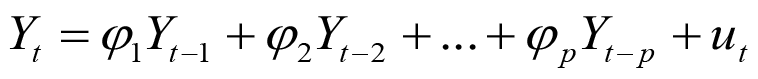
ARIMA model is a most suitable form of stochastic models analyzing the stationary time series data. Usually data of time series are non stationary, by taking the difference of the time series data is converted easily into stationary. ARIMA model is the combination of autoregressive (AR) term, integrated (difference) term and moving average (MA) term, it is denoted by ARIMA (p, d, q) model, where p, d and q denote orders of auto-regressive (AR) model, difference and moving average (MA) model respectively. Generally autoregressive model of order (p) is of the form:
Order of the difference “d” suggested through the Augmented Dickey Fuller (ADF) unit root test (1979) as.
Zt = Yt -Yt -d
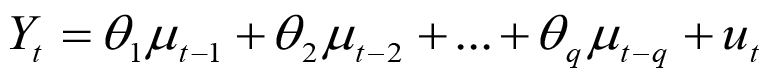
While moving average model of order (q) is of the form:
Then, the ARIMA (p, d, q) is:

Where;
Yt is the production of fisheries at time t. Yt-1, Yt-2, Yt -3,…..Yt-p are the lag values at time t-1 , t-2 .…..t-p respectively. ut, ut-1....... ut-q, are the error terms and its lag values, while the φ1 ……..φp are the coefficients of autoregressive model and θ1 …….θq are the coefficients of moving average model.
Table 3: Estimates of parameters of the ARIMA (2,1,3) models.
| Type | Coefficient | S.E( Coef) | t(test) | P-value |
| AR(1) | -1.5380 | 0.2347 | -6.55 | 0.000 |
| AR(2) | -0.7454 | 0.1541 | -4.84 | 0.000 |
| MA(1) | -1.4794 | 0.1849 | -8.00 | 0.000 |
| MA(2) | -0.6964 | 0.1053 | -6.62 | 0.000 |
| MA(3) | 0.1463 | 0.0731 | 2.00 | 0.050 |
| Constant | 27.789 | 9.911 | 2.80 | 0.007 |
Table 4: Forecast from year 2013-14 to year 2025-26 at 95% limits.l
| Periods | Forecast | Lower limit | Upper limit | Actual | % forecast error |
| 2013-14 | 625.876 | 573.031 | 678.721 | 623.022 | -0.4560% |
| 2014-15 | 616.491 | 543.914 | 689.068 | 623.457 | 1.1299% |
| 2015-16 | 648.648 | 559.413 | 737.884 | 643.164 | -0.8454% |
| 2016-17 | 633.974 | 534.851 | 733.097 | ||
| 2017-18 | 660.362 | 546.995 | 773.729 | ||
| 2018-19 | 658.504 | 537.146 | 779.861 | ||
| 2019-20 | 669.481 | 537.264 | 801.697 | ||
| 2020-21 | 681.772 | 541.416 | 822.128 | ||
| 2021-22 | 682.474 | 533.964 | 830.984 | ||
| 2022-23 | 700.021 | 543.212 | 856.829 | ||
| 2023-24 | 700.299 | 536.742 | 863.855 | ||
| 2024-25 | 714.580 | 543.239 | 885.921 | ||
| 2025-26 | 720.196 | 542.551 | 897.841 |
Results and Discussion
Time plot for the production of the fisheries shows the trend, which indicate the original series is non stationary, to make the stationary of the series graphs of autocorrelation function (ACF), partial autocorrelation function (PACF), and augmented dickey-fuller (ADF) of unit root test is constructed.
The stationary of the data is tested by both graphs and augmented dickey-fuller (ADF) unit root test. From the graphs of autocorrelation function (ACF), partial autocorrelation function (PACF), and augmented dickey-fuller (ADF) of unit root test, first difference is necessary to make the stationary of the above series. First order difference, Zt = Yt -Yt -1 is taken from the observed data series of the fisheries production.
Graph of first difference of the original fisheries production shows the stationary of the data.
There is no negative spike in the graph of autocorrelation function, zero order of moving average (MA) model is suggested, and there is one positive spike in the graph partial autocorrelation function, first order of autoregressive (AR) model is considered. So, tentative autoregressive integrated moving average (ARIMA) model is ARIMA (1, 1, 0) is used. In this study best forecast ARIMA (p, d, q) model is chosen by comparing all possible fitted model diagnostically starting from ARIMA (1, 1, 0).
Mean square error is minimum and value of R-Square for the ARIMA (2, 1, 3) model is better than the other all possible ARIMA models. Box-Pierce (Ljung-Box) chi-square statistic is satisfy for the proposed model. Parameters of ARIMA (2, 1, 3) model given in Table 3 are also significant. As the series become stationary after the difference of first order, therefore it is written with the help of back shift operators.


By adding the constant term, it can be written as follows.

After comparing all possible models ARIMA (2, 1, 3) is proposed as a best forecast model for fisheries production. Graphically diagnostic checks of ARIMA (2, 1, 3) model in the Figures 7 and 8 are the residual plot for the autocorrelation and partial autocorrelation functions, which shows that all of the autocorrelations and partial autocorrelations lie between the 95% confidence interval. Normal probability plot for residuals in Figure 9 shows that the residuals lie along a straight line. From all the diagnostic checks the model is parsimonious and correctly specified.
After specification of the adequate model it is necessary to utilize it for forecasting the fisheries production. In forecasting objective of research is to predict the future values of the fisheries production for the year 2017-2026. Figure 10 shows the time plot for the forecast values of fisheries production and table number 4 provide the forecast values for the year 2017-2026 at 95% confidence interval.
Conclusions and Recommendations
Forecasting results of ARIMA (2, 1, 3) model, suggested through Box-Jenkin’s Methodology are best for forecasting the production of fisheries for the year 2017-2026. Forecasting accuracy and comprehensiveness of different ARIMA models are also supported by Amin et al. (2014), Senol (2015) and Şenol and Sengul (2018). Forecast error -0.4560, 1.1299 and -0.8454 percent is very minimum for the proposed model. These forecasting results show a significant increase, from 619.624 to 724.750 tons of fisheries production from the year 2017-2026. The prediction of this study may provide help to policy makers make their macro-level policies for food security, better planning for the fisheries production and fish export policies to earn more national income. It also provides help, micro level policies for marine and inland fish production, to solve the problem of the coastal population of the Pakistan. Proposed ARIMA (1, 1, 0) model for forecasting is recommended for government exports, researchers, business men, and fish producers for information and planning their resources as well as decision making regarding the production of fisheries in Pakistan.
Author’s Contribution
Qaisar Mehmood: Idea, complete write up and management of the research.
Maqbook Hussain Sial and Saira Sharif: Help in discussion of the results.
Abid Hussain: Help in data in selection of data.
Muhammad Riaz and Nargis Shaheen: Help in model fitting
References
Allen, P.G., 1994. Economic forecasting in agriculture. Int. J. Forecasting. 10(1): 81-135. https://doi.org/10.1016/0169-2070(94)90052-3
Bahnasawy, M., A.A. Khidr and D. Nadia. 2009. Seasonal variations of heavy metals concentrations in mullet, Mugil cephalus and Liza ramada (Mugilidae) from Lake Manzala, Egypt. J. Appl. Sci. Res. 5(7): 845-852.
Bajpai, P.K. and R. Venugopalan. 1996. Forecasting sugarcane production by time series modeling. Indian J. Sugarcane Technol. 11(1): 61–65.
Boken, V.K., 2000. Forecasting spring wheat yield using time series analysis. Agron. J. 92(6): 1047-1053. https://doi.org/10.2134/agronj2000.9261047x
Box, G.E.P. and G.M. Jenkins. 1976. Time series analysis. Forecasting Control, Revised Ed, Holden Day.
Dickey, D.A. and W.A. Fuller. 1979. Distribution of the estimators for autoregressive time series with a unit-root. J. Am. Stat. Assoc. 74: 427-431. https://doi.org/10.1080/01621459.1979.10482531
GOP. 2016. Pakistan economic survey, finance division, economic advisor’s wing, Islamabad.
Karunarathna, B. and K.A.N.K. Karunarathna. 2017. Forecasting fish production in Sri Lanka by using ARIMA model. Scholar J. Agric. Vet. Sci. 4(9): 344-349.
Masood, M.A. and M.A. Javed. 2004. Forecast models for sugarcane in Pakistan. Pak. J. Agric. Sci. 41(1-2): 80-85.
Muhammad, F., M.S. Javed and M. Bashir. 1992. Forecasting sugarcane production in Pakistan using ARIMA Models. Pak. J. Agric. Sci. 9(1): 31-36.
Pakistan Bureau of Statistics. Agricultural statistics. 50 years of Pakistan: volume-iii (1947-1997).
Retnam, A. and M.P. Zakaria. 2010. Hydrocarbons and heavy metals pollutants in aquaculture. http://psasir.upm.edu.my/id/eprint/5601/1/5.pdf.
Şenol, C., 2015. Estimation of Number of Small Cattle through ARIMA Models in Turkey. J. Math. Syst. Sci. 5: 464-473. https://doi.org/10.17265/2159-5291/2015.11.003
Tsitsika, E.V., C.D. Maravelias and J. Haralabous. 2007. Modeling and forecasting pelagic fish production using univariate and multivariate ARIMA models. Fish. Sci. 73: 979–988. https://doi.org/10.1111/j.1444-2906.2007.01426.x
Venugopalan, R., and M. Srinath. 1998. Modeling and forecasting fish catches: Comparison of regression, univariate and multivariate time series methods. Indian J. Fish., 45(3): 227–237.
World bank. 2016. Fisheries statistics, World Development indicators.
Yaseen, M., M. Zakriya, I.D. Shahzad, M.I. Khan and M.A. Javed. 2005. Modeling and forecasting the sugarcane yield of Pakistan. Int. J. Agric. Biol. 7: 180-183.