INTRODUCTION
Sheep raising is one of the main activities of Peruvian livestock producers, mainly in the Puno region, where the largest population of sheep is found. Around 25.48% of sheep in Peru are located in the Puno region and are mainly raised by smallholders in extensive systems, grazing on natural grasslands (MIDAGRI, 2021). The decline in meat and wool prices as a result of inadequate technical support, migration from rural to urban areas, limited use of technology and inefficient use of natural rangelands is continuing. An efficient strategy for managing herds which includes consistent assessment of production traits, like assessing body weight and composition, could aid struggling producers.
Body weight of farm animals is the most essential trait in the herd’s productive efficiency, mainly for meat production. This trait allows producers to assess the general condition of animal, can be used as a basis for selection in animal improvement programs, used to formulate balanced diets, health management, and to decide when the fattening period is complete, among others ; . Therefor body weight must be estimated with high accuracy, but can be difficult without suitable equipment, which can be expensive and difficult to transport.
Fortunately, it has been published that there is an important relationship between live weight and body measurements of sheep (Canaza-Cayo et al., 2017, 2021), goats , and cows . Therefore, various statistical regression models have been suggested to estimate live weight based on measurements of body dimension ; Canaza-Cayo et al., 2017, 2021; . Nevertheless, when there are many predictor variables, multicollinearity arises among them, resulting in the problem of overfitting . In general, multiple linear regression (MLR) analysis is widely used to estimate the body weight of animals based on biometric measures.
The MLR using stepwise selection method, also known as stepwise regression (SR) is a statistical technique of choosing variables of interest from several other variables in the regression model. As the initial step, whole explanatory variables incorporated in linear equation, then, in each subsequent step, the least significant variable with the highest p-value eliminated . However, SR can generate unreliable parameter estimates in situations where the number of predictors is greater. Alternatively, ridge regression (RR) analysis is a helpful tool to overcome multicollinearity due to strong bivariate-correlations between independent variables. Insignificant variables can be reduced so their coefficients approach zero through an added constraint. The constant ‘k’ is established using a variance inflation factor and a ridge trace .
To the best of our knowledge, little research has been reported about predicting body weight via Ridge Regression in Corriedale sheep. Thus, the purpose of this study was to predict body weights of Corriedale ewes from various body measurements using stepwise and ridge regression models.
MATERIALS AND METHODS
Study area and data collection
Records of 100 female Corriedale sheep aged 1.5 to 2 years were utilized in the study. The animals were housed at the Illpa Experimental Center from National University of Altiplano, located in the Puno Department of Peru. Body weight (BW) and body measurements (BM) including, body length (BL), abdominal perimeter (AP), rump height (RH), wither height (WH), thoracic perimeter (TP), loin width (LWi), tail perimeter (TPe), hip width (HW), fore-shank width (FSW), tail width (TW), shoulder width (SW), forelimb length (FL), fore-shank length (FSL) and fore-shank perimeter (FSP) were recorded. BW was obtained using a weighing scale in kg, while a wood ruler and a centimeter-long measuring tape were used to measure the BM.
Statistical Analysis
(MLR) analysis is a statistical method used for modeling the relationships between variables, including both response and explanatory variables (Montgomery et al., 2012). A MLR in matrix formula may be written as:

Where y is represent a (n x 1) column vector of records associated with the response variable, X is a (nxp) incidence matrix of records of the explanatory variables, 

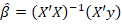
 estimator of the parameters is obtained by applying equation 2 :
In the present research, BW was the response variable, while the ’s parameters for BM were utilized as predictor variables. To address the problem of multicollinearity between the explanatory variables, this study utilized stepwise regression (SR) and ridge regression (RR) analysis.
Stepwise regression analysis
SR is a method of selecting a subset of predictor variables for a regression model, from a wide range of potential explanatory variables. In the first step, all predictors were included in the model. Each step involved removing the least significant predictor with the highest p-value. This method includes three main variations: forward selection, backward elimination, and stepwise. In forward selection, the model begins with no predictors and consecutively adds significant ones until meeting a statistical stopping criteria. In backward elimination, the model begins with all potential predictors and gradually removes those that are non-significant until meeting a statistical stopping criteria. Stepwise regression (SR) blends both approaches, adding and removing predictors as it builds the model . The SR analysis was performed using the MASS package of software R (R Core Team, 2023).
Ridge regression analysis
Ridge regression (RR) is a statistical technique used to address multicollinearity and prevent issues related to small sample sizes and a high number of predictor variables. When multicollinearity is present, OLS estimates remain unbiased, but their variances are high, which can cause them to deviate significantly from the true value. Ridge regression introduces a degree of bias to the regression estimates, thereby reducing standard errors. The expectation is that this will lead to more reliable estimates overall (Hastie et al., 2001).
The ridge estimator

where k is ridge parameter determined as a positive number and I denote an identity matrix. The RR analysis was performed using the lmridge package of software R (R Core Team, 2023).
Assessment of prediction accuracy
Different Goodness-of-fit metrics were used to evaluate the performance of the models used to predict the ewes’ body weight. Among them, the coefficient of determination (R2), Pearson coefficient of correlation (r), root mean square error (RMSE), means square error (MSE), mean absolute deviation (MAD), mean absolute error (MAE) and mean absolute percentage error (MAPE). The model with the least RMSE, MSE, MAD, MAE and MAPE values and high R2 values in training and testing datasets was selected as the best model to predict the BW of Corriedale ewes. The goodness-of-fit metrics analysis was performed using the Metrics package of software R (R Core Team, 2023).
RESULTS AND DISCUSSION
Table 1 shows descriptive statistics for body weight and linear body measurements of Corriedale ewes. BW varied between 22 and 66 kg, with a mean of 34.39 kg and a standard deviation of 4.68 kg. The coefficient of variation for body measurements ranged from 4.35% (RH) to 18.08% (TPe).
Pearson correlation between body measurements and BW
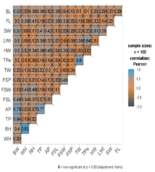
Figure 1 presents Pearson’s correlation coefficients among the body measurements, including body weights (BW), across the entire dataset. Overall, a high positive correlation (P < 0.05) was observed between BW and AP (0.78), while a moderate positive correlation (P < 0.05) was found between BW and TP (0.64), HW (0.50), LWi (0.50), SW (0.51), and BL (0.52). There was a weak positive correlation among BW and other body measurements (≤ 0.48, P > 0.05). Çakmakçı (2022) observed comparable patterns in Norduz ewes and discovered a high correlation between BW and TP (0.87). Canaza-Cayo et al. (2021) in Corriedale ewes and Faraz et al. (2023) in Kajli sheep also reported higher correlations between BW and AP.
The results in the present study also showed that there was a significant and very high relationship (P<0.05) between WH and RH (0.93) while a high correlation between TP and AP (0.77), and between TW and TPe. A positive and moderate correlation (P<0.05) between TPe and LWi (0.64) and between HW and SW (0.61) was also observed. The other body measurements showed low (P<0.05) to very low magnitude (P>0.05) correlations, with values ranging from 0.23 to 0.49. Little research has been reported on Pearson’s correlations among different body measurements in sheep. The results of the present study were consistent with those published for the Corriedale, Kajli, and Santa Inês breeds by Canaza-Cayo et al. (2021), Faraz et al. (2023), and Gurgel et al. (2021), respectively.
Stepwise regression
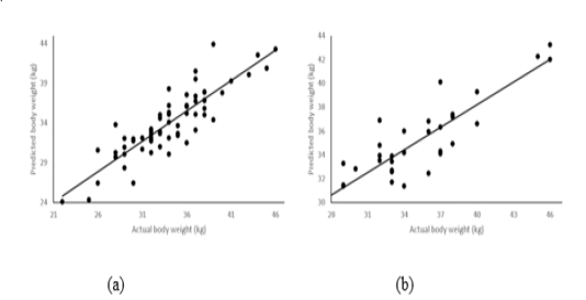
The stepwise regression analysis results are presented in Table 2. Results indicated that the AP, FSL, HW, LWi and BL were significant predictor variables included in the model with an R2 = 0.76 to predict body weight of Corriedale ewes. In addition, according to VIF, no multi-collinearity was found between the predictor variables (VIF>10, . The current study’s findings align with those published by Canaza-Cayo et al. (2021). The body weight of the Corriedale ewes was predicted using equation 4 (next paragraph), established by the stepwise regression analysis; allowing us to compare the predicted body weight with the actual body weight at a 95% confidence interval (Figure 2).
Table 1: Descriptive statistics of body weight (kg) and body measurements (cm) of Corriedale ewes.
| Traits | Mean | Median | SD | Min | Max | CV(%) |
| BW | 34.39 | 34.0 | 4.68 | 22 | 46 | 13.62 |
| WH | 59.80 | 60.0 | 2.68 | 50 | 66 | 4.49 |
| RH | 61.08 | 61.0 | 2.66 | 52 | 68 | 4.35 |
| TP | 82.55 | 81.0 | 4.4 | 72 | 99 | 5.33 |
| AP | 96.96 | 97.0 | 5.57 | 80 | 112 | 5.74 |
| FSL | 20.41 | 20.0 | 1.25 | 17 | 25.5 | 6.14 |
| FSW | 2.51 | 2.5 | 0.34 | 2 | 3 | 13.75 |
| FSP | 8.43 | 8.5 | 0.59 | 6 | 10 | 7.05 |
| TW | 3.17 | 3.0 | 0.52 | 2.5 | 5 | 16.36 |
| TPe | 7.45 | 7.0 | 1.35 | 6 | 17 | 18.08 |
| HW | 19.38 | 20.0 | 1.6 | 11 | 23 | 8.24 |
| LWi | 12.46 | 12.0 | 1.01 | 10 | 18 | 8.12 |
| SW | 19.33 | 19.5 | 1.44 | 15 | 23 | 7.46 |
| FL | 37.06 | 37.0 | 2.41 | 27 | 42 | 6.51 |
| BL | 95.48 | 96.0 | 4.28 | 83 | 104 | 4.48 |
SD: standard deviation; CV: coefficients of variation; BW: body weight; WH: wither height; RH: rump height; TP: thoracic perimeter; AP: abdominal perimeter; FSL: fore-shank length; FSW: fore-shank width; FSP: fore-shank perimeter; TW: tail width; TPe: tail perimeter; HW: hip width; LWi: loin width; SW: shoulder width; FL: forelimb length and BL: body length.
Table 2: Estimated stepwise regression parameters, significance level, tolerance and VIF values obtained from training dataset.
| Variable | B | SE | t | Pr(>|t|) | Sig | VIF |
| Intercept | -59.20 | 7.21 | -8.21 | 0.00 | *** | |
| AP | 0.37 | 0.07 | 5.23 | 0.00 | *** | 1.93 |
| FSL | 0.58 | 0.24 | 2.42 | 0.02 | * | 1.27 |
| HW | 0.60 | 0.23 | 2.61 | 0.01 | * | 1.68 |
| LWi | 0.83 | 0.32 | 2.55 | 0.01 | * | 1.46 |
| BL | 0.25 | 0.07 | 3.44 | 0.00 | ** | 1.26 |
AP: abdominal perimeter; FSL: fore-shank length; HW: hip width; LWi: loin width; BL: body length, SE: standard error. VIF: variance inflation factor, B: regression parameter, t: t-test statistics. Significance codes: *** 0.001 ** 0.01 * 0.05
Table 3: Goodness-of-fits metrics for different K Ridge estimators for training and testing dataset
| K | Training dataset | Testing dataset | |||||||
| MSE | PRESS | R2 | AIC | MSE | PRESS | R2 | AIC | ||
| 0.00 | 411.19 | 689.67 | 0.79 | 131.36 | 274.30 | 384.05 | 0.86 | 61.94 | |
| 0.25 | 215.06 | 527.72 | 0.66 | 126.49 | 83.72 | 232.02 | 0.70 | 55.89 | |
| 0.50 | 264.82 | 521.86 | 0.58 | 127.94 | 93.33 | 233.42 | 0.59 | 57.32 | |
| 0.75 | 299.03 | 529.28 | 0.52 | 130.13 | 107.71 | 245.09 | 0.51 | 59.53 | |
| 1.00 | 324.44 | 541.90 | 0.47 | 132.58 | 120.90 | 259.42 | 0.45 | 61.79 | |
| 1.25 | 344.63 | 557.18 | 0.43 | 135.10 | 132.49 | 274.43 | 0.40 | 63.93 | |
| 1.50 | 361.41 | 573.92 | 0.39 | 137.60 | 142.71 | 289.37 | 0.36 | 65.91 | |
| 1.75 | 375.79 | 591.43 | 0.36 | 140.03 | 151.79 | 303.87 | 0.32 | 67.72 | |
| 2.00 | 388.40 | 609.29 | 0.33 | 142.36 | 159.95 | 317.79 | 0.29 | 69.37 | |
MSE: Mean square error; PRESS: Predicted residual error sum of squares; R2: coefficient of determination, AIC: A kaike information criterion
Table 4: Ridge regression parameters, standard errors and VIF values for training data
| Variable | B | B* | SE* | t* | Pr(>|t|) | Sig | VIF* |
| Intercept | -61.40 | -2656.61 | 385.66 | -6.89 | 0.00 | *** | |
| WH | 0.05 | 1.03 | 1.75 | 0.59 | 0.56 | 0.50 | |
| RH | 0.17 | 3.73 | 1.68 | 2.22 | 0.03 | * | 0.47 |
| TP | 0.08 | 2.90 | 2.15 | 1.35 | 0.18 | 0.76 | |
| AP | 0.25 | 11.66 | 2.17 | 5.38 | 0.00 | *** | 0.77 |
| FSL | 0.50 | 5.61 | 2.09 | 2.69 | 0.01 | ** | 0.71 |
| FSW | -0.57 | -1.56 | 2.13 | -0.73 | 0.47 | 0.75 | |
| FSP | 0.57 | 3.00 | 2.08 | 1.44 | 0.16 | 0.71 | |
| TW | 0.47 | 2.17 | 1.93 | 1.13 | 0.26 | 0.61 | |
| TPe | 0.01 | 0.10 | 1.74 | 0.06 | 0.96 | 0.50 | |
| HW | 0.39 | 5.29 | 2.07 | 2.55 | 0.01 | * | 0.71 |
| LWi | 0.51 | 4.50 | 2.09 | 2.15 | 0.04 | * | 0.72 |
| SW | 0.26 | 3.00 | 2.13 | 1.41 | 0.16 | 0.74 | |
| FL | -0.03 | -0.70 | 2.07 | -0.34 | 0.74 | 0.71 | |
| BL | 0.20 | 7.39 | 2.10 | 3.52 | 0.00 | *** | 0.73 |
WH: wither height; RH: rump height; TP: thoracic perimeter; AP: abdominal perimeter; FSL: fore-shank length; FSW: fore-shank width; FSP: fore-shank perimeter; TW: tail width; TPe: tail perimeter; HW: hip width; LWi: loin width; SW: shoulder width; FL: forelimb length and BL: body length, SE*: standardized standard error. VIF*: standardized variance inflation factor, B: regression parameter, B*: standardized regression parameter t*: standardized t-test statistics.
Significance codes: *** 0.001 ** 0.01 * 0.05
Table 5: Goodness-of-fit criteria for comparing the model performances.
| Criteria | Stepwise regression model | Ridge Regression model | |||
| Training dataset | Test dataset | Training dataset | Test dataset | ||
| RMSE | 2,277 | 2,358 | 2,251 | 2,609 | |
| MSE | 5.186 | 5.560 | 5.069 | 6.804 | |
| MAD | 1,788 | 1,947 | 1,810 | 2,185 | |
| MAE | 1,788 | 1,947 | 1,810 | 2,185 | |
| MAPE | 5,319 | 5,583 | 5,342 | 6,156 | |
| r | 0,873 | 0,865 | 0,879 | 0,842 | |
| R2 | 0,842 | 0,730 | 0,768 | 0,669 | |
R2: coefficient of determination, r: Pearson coefficient of correlation, RMSE: root mean square error, MSE: means square error, MAD: mean absolute deviation, MAE mean absolute error, MAPE: mean absolute percentage error.
In the stepwise regression, the variables WH, RH, TP, FSW, FSP, TW, TPe, SW, FL and RHI were evaluated and eliminated from the model after evaluating their contributions. The final model (Table 3) identified after seven steps had an R² of 0.76, AIC of 314.4 and RMSE of 2.28 kg and resulted in equation 4:


Ridge regression
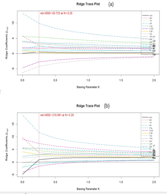
The results of Goodness-of-fit metrics for different K Ridge estimators on both the training and testing datasets are given in Table 3. The best K value was 0.25 attributable to the smallest MSE, PRESS and AIC values and the highest R2 value for training and testing dataset. It shows that at K = 0.25 stability was achieved in all the body measurements; having eliminated collinearity, as demonstrated by the ridge trace plot (Figure 3).
The findings of Ridge regression analysis are given in Table 4. Results indicate that the AP, FSL, HW, LWi and BL were the significant predictor variables included in the model with R2 = 0.76 to predict body weight of Corriedale ewes. In addition, according to VIF, no multi-collinearity was found between the predictor variables (VIF>10, .
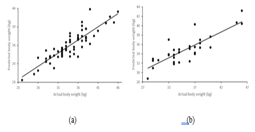
Predictive performance results of stepwise (SR) and ridge regression (RR) models and goodness-of-fit criteria of Corriedale ewes, are displayed in Table 5 and Figure 4. The SR model had the highest R2 value and the lowest values of MAD, MAE, and MAPE on the training dataset. However, the RMSE and MSE of the RR model were higher than the SR model. SR outperformed the RR model with higher R2 values and smaller values of RMSE, MSE, MAD, MAE, and MAPE based on the testing dataset. These differences may be due to sampling variance in both the training and testing data sets. Overall, these results are in agreement with other studies in sheep, reporting the better goodness-of-fit criteria in the training dataset than the testing dataset ; ; ; .
CONCLUSIONS
In this research, we carried out a comparative analysis of SR and RR models for predicting the body weight of Corriedale sheep. Both SR and RR models provide good results but the SR model was slightly superior to the RR model. Therefore, we recommend the SR model whose prediction equation is:


ACKNOWLEDGEMENTS
The authors are thankful for the valuable support from all staff of the Illpa Experimental Centre at the National University of Altiplano, Puno Peru. For the phenotypic data collection. We also thank to Coordenação de Aperfeiçoamento dePessoal de Nível Superior (CAPES) for the financial support granted to the first author.
CONFLICT OF INTEREST
There were no conflicts of interest.
NOVELTY STATEMENT
In this research the live weight of Corriedale sheep was predicted using stepwise and ridge regression from fourteen independent variables.
AUTHORS CONTRIBUTIONS
Roxana Churata-Huacani; Writing of Original draft, Writing, Review and Editing. Ali William Canaza-Cayo; Conceptualization, Formal analysis. Tales Jesus Fernandes, Júlio Sílvio de Sousa Bueno Filho; Writing, Review and Editing.