Research Article

Forecasting Area and Production of Guava in Pakistan: An Econometric Analysis

Dilawar Khan1*, Arif Ullah2, Zainab Bibi1, Ihsan Ullah1, Muhammad Zulfiqar4 and Zafir Ullah Khan3

1Department of Economics, Kohat University of Science and Technology, Kohat 26000, Khyber Pakhtunkhwa, Pakistan; 2Department of Economics, Preston University Kohat Campus, Kohat 26000, Khyber Pakhtunkhwa, Pakistan; 3Department of Economics, University of Science and Technology, Bannu 28100, Khyber Pakhtunkhwa, Pakistan; 4Institute of Development Studies, The University of Agriculture, Peshawar, Khyber Pakhtunkhwa, Pakistan.

Received | September 21, 2019; Accepted | December 01, 2019; Published | February 20, 2020

*Correspondence | Dilawar Khan, Associate Professor, Department of Economics, Kohat University of Science and Technology, Kohat 26000, Khyber Pakhtunkhwa, Pakistan; Email: dilawar@kust.edu.pk

Citation | Khan, D., A. Ullah, Z. Bibi, I. Ullah, M. Zulfiqar and Z.U. Khan. 2020. Forecasting area and production of guava in Pakistan: An econometric analysis. Sarhad Journal of Agriculture, 36(1): 272-281.

DOI | http://dx.doi.org/10.17582/journal.sja/2020/36.1.272.281

Keywords | Forecasting, Area, Production, Guava, The Box-Jenkins approach

Introduction

One of the core objectives of United Nation (UN) is to diminish global poverty and hunger. For this reason, UN has set fundamental objectives in the shape of Millennium Development Goals (MDGs). The increase in the world population has been projected that at the end of year 2050 it would be around 9.3 billion and the immense increase in Pakistan’s population is being expected in coming decades (UN, 2011). Population of Pakistan currently 20.6 million and expected to increase 300 million in 2050 (GOP, 2019). The immense population growth needs more food and greater amenities of life. Over a long period of time agriculture sector was responsible for Pakistan’s growing population to ensure food security. The agriculture sector plays a vitale role in Pakistan’ economic growth and contributes 19.8% to national income. This sector also provides oppertunities of employment and generate an account of 42.3% labour force (GOP, 2016).

Horticultural crops play a significant role in balancing human diet. These crops on one hand provide energy-rich food and on the other hand also promise supply of essential protective nutrients. Pakistan’s region has rich topographic and climatic endowments on which horticultural crops are grown in large number. These include vegetables, fruits, tuber crops, roots, medicinal, ornamental and plantation crops, aromatic plants and spices (Ullah et al., 2017). In recent times considerable export earnings were gained from horticultural production. Specifically, per year 12 million tonnes of horticultural products are grown in Pakistan. These includes fruits, vegetables and spices. Therefore, this sector has the capability to eradicate poverty and reduce issues of socio-economic of the country (PHDEC, 2017).

Guava (Psidium guajava L.) belongs to family Myrtaceae. It is a tropical fruit widely relished in the tropics. This fruit hold third position among fruits area and production. Mature and freshly plucked guava has a sweet and attractive flavour. It is largely eaten fresh but is also used in jams and jellies. It has water, protein, and carbohydrate 82%, 0.7% and 11% respectively. Further it is also considered as a rich source of A, B and C vitamins. In terms of more nutritionally it is useful source of soluble fibre, phosphorous, nicotinic acid and calcium. An average guava contains about 25 calories. It has good nutritional value (Khushk et al., 2009).

There are two (winter and summer) seasons of guava fruit in Pakistan. The winter season begins from November till March and the summer from April to the middle of August. Among the guava major producing countries Pakistan is the second largest guava producing nation. It is extensively grown in various parts of Pakistan. In Sindh province it is cultivated in Larkana and Hyderabad districts. In Punjab province it is extensively grown in Lahore, Sharaqpur Sharif, Kasur, Gujranwala and Sangla Hills districts. Moreover, district Kohat of Khyber Pakhtunkhwa is recognized due guava quality and quantity production. In addition, Haripur and Bannu districts of Khyber Pakhtunkhwa province also cultivate this fruit. Its total cultivated area was 65.6 thousand hectares and production 489.1 thousand tons during the year 2014-15 (GOP, 2015).

The uncertainty of future agricultural production and consumption level makes agricultural production strategy and investment planning difficult. Forecasts of agricultural production within the specified production conditions provide necessary information to carry out production and investment planning process. Guava is an important fruit in Pakistan. Using the past trends, it is necessary to check the future aspects of this fruit. With the best of our knowledge, none of the researchers have investigated the taken the case of guava in Pakistan. Researchers, economist, planner, producer and businessman always take interest in the latest figures and updates of future status of guava in Pakistan. Therefore, it is a dire need to provide update regarding future aspects of this fruit. The rest of the manuscript is structured as follow. The next section presents materials and methods and results and discussions are presented in the third sections. Final section concludes the results of the study.

Materials and Methods

This research study is based on the Box-Jenkins (1976) approach and time series data was used over the time span of 1997-98 to 2014-15. The aim of this manuscript is determined the Pakistan guava area and production using forecasting technique of ARIMA model. The data was taken for both the series from Agricultural Statistics of Pakistan (GOP, 2015). ARIMA modelling approach was adopted and with the help of econometric software E Views version 9 for the forecasting of guava area and production analyses were carried out. Using this approach guava area and production forecast was made up to the period 2029-30.

Refers to the literature of time series there is quite difference between classical modeling. These models are exponential smoothing and Box-Jenkins approach. Exponential smoothing techniques are established purposively because it does not require probabilistic reasoning. In the time series it uses the idea of weight distribution to consider time-varying weights. The behavior of a particular time series is represented through a little intuitive way called smoothing. This means a moving average process considering the application of autoregressive models (defined by previous values and addition of noise). However, it use the terms autoregressive and moving average simultaneously. Therefore, such combination characterized as ARMA model (Autoregressive Moving Average). Stationarity is the process to make the series stationary. This can be made through differentiation. ARIMA model is the integrated order of two parts. The first part is called Autoregressive, while second is known as Moving Average.

Generally, there are four main steps in ARIMA modelling. First is the identification step. Using the AIC criteria, the estimation and identification may overlap. Therefore, trial-and-error fitting requires for the estimated model. The model fitness and its diagnosis are performed in second and third step. The diagnostic step shows the model fitness. Forecasting of the series is performed in the final step. This methodology has been employed by a number of researchers to forecast production, consumption, imports and exports of foods and non-food items. The most similar work in this area was done by Rahman and Baten (2016) for Bangladesh and Badmus and Ariyo (2011) for Nigeria. In both study’s authors have used the ARIMA model respectively for their respective countries. Moreover, Ahmad et al. (2005) employed the same method to predict the growth trends of Kinnow’ production and export in Pakistan while Ahmad and Mustafa (2006) used the same approach to investigate the future aspect of Kinnow. In the similar context, Qureshi et al. (2014) have forecasted the production of citrus fruit in Pakistan using ARIMA model. Furthermore, Jam et al. (2013) and Khan et al. (2008) contributed in the similar literature and found out future aspect of mango in Pakistan. More research work was done to forecast area for instance Ullah et al. (2018) in Pakistan, Suleman and Sarpong (2012) in Ghana, Iqbal et al. (2000), Saeed et al. (2000), Amin et al. (2014) and in Pakistan. In all these studies ARIMA model was used for the forecasting of various agriculture commodities.

Furthermore, similar research was done by Boken (2000) in Canada. The author applied various model using wheat yield time series data. The author concluded that quadratic model is the ideal method for forecasting wheat yield. However, based on stochastic criteria, the author concluded that simple average model is appropriate. Accordingly, Sabir and Tahir (2012) used the time series data for forecasting wheat’ area and production. The exponential smoothing method was used to accomplish the objective of the research. It was concluded that in the year 2011-12 for the population of 97.67 million 12.70 million tons of wheat production would be required. Jambhulkar (2013) investigated the ARIMA approach to forecast rice production in India using time series data for the period of 1960-1961 to 1999-2000.

ARIMA is considered one of the best choices due to its standard procedure and technique developed by the Box-Jenkin (1976). The development of the ARIMA model refers to the set of procedures. The first step is the identification of the model. Next is the parameter estimation. The third step is the diagnostic verification of the model. The final stage is the forecasting stage. Here the best fit model is selected. The first component of the time series ARIMA identifies as pth order of AR (p) and mathematically it can be expressed as follow.

 

Where;

φ0, φ1, φ2,.……. , φp are parameters to be estimated in the model, ɛt is residual term at time “t”, Rt indicates dependent variable in the model with respect to time “t” and Rt-1+ Zt-2, …., Rt-p is dependent variable at time period i.e. t-1, t-2, …., t-p lags. The second component of the time series ARIMA is defined as moving average (MA) model of qth order MA (q). The mathematical expression of MA (q) is presented with the following regression.

 

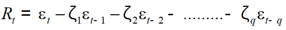
Where;

ɛt is the residual term in the model at a time t. The estimated coefficients of the model are denoted as ζ1, ζ 2 , .……., ζq. The dependent variable is also called response variable presented as Rt at time “t”. The response variable (Rt) error is shown as ɛt-1, ɛt-2, …….., ɛt-q. The first component AR (p) and second component MA (q) jointly form ARMA model. However, by integrating these two components it becomes ARIMA and mathematically can be specified as follow.

Whereas the integrated component can be expressed with the term d shows the order of differencing of Rt. The general format of the this model is written as ARIMA (p, d, q) (Anderson, 1971).

The most important issue in ARIMA modelling technique is the identification of p, q and d adequate values. Moderately, this issues can be overcome through by using the autocorrelation (AC) and partial autocorrelation (PA) functions, pattern and sequence of the residual or processed series (Pindyck et al., 1991). Nonetheless, for the identification of any ARIMA (p, d, q) model, the theoretical partial autocorrelation function for AR(p) model has non-zero valued parameters at all lags; 1, 2, …, p and has zero-valued parameters at all lags. The theoretical autocorrelation function for MA(q) has non-zero valued parameters at all lags; 1, 2, …, q and zero-valued parameters at all lags. The non-zero lags of the sample partial autocorrelation function and autocorrelation function are tentatively accepted as the p and q parameters of the models. To achieve the stationarity of the series, the differencing approach is used if the original series as non-stationary series. Where “d” identifies is the difference operator. Consequently, when a series is stationary at the level then ARIMA (p, d, q) can be reduced to ARMA (p, q) with the order of differencing term becomes equal to zero (d = 0).

To perform time series analysis, the stationary test is a necessary process. To remove the problems of stationarity we employed and Phillips-Perron, 1988 (PP) test. The inclusion of the PP unit root test in the study is because of the two reasons. First to detect the serial correlation with in the data. Second, it has the capability to show robustness over time dependent heteroscedasticities. However, to choose the appropriate lag length of ADF and PP test, the minimum value of model selection criteria is used.

ARIMA models are fitted and the accuracy of the model was tested on account of diagnostics statistics. The best and an appropriate ARIMA model is selected using the following diagnostics. To choose the ideal ARIMA model, the study employs three model selection criteria, namely AIC (Akaike Information Criterion), SIC (Schwarz Information Criterion) and the HQ (Hannan-Quinn Criterion). These criteria measure the adjustment between the uncertainty and the number of parameters included in the model. The best and true ARIMA model is select based on the lowest value of these criteria. The econometric equations of AIC, BIC and HQ can be estimated using the following formula:

 

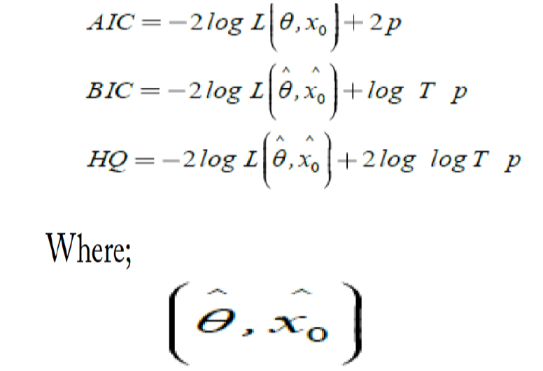
are the maximized values and p gives the number of parameters in θ̑ plus the number of the estimated initial states in x̑0. The model that minimizes the AIC, BIC and HQ across all available models is adopted. The insignificance of autocorrelations for residual describes as if a model is a suitable depiction of time series, it would test the correlation problem and residuals should be independent of another. Finally, future values of the time series were forecasted.

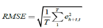
The quality and predictability power of the models and measures of forecast accuracy depends on a number of criteria. The first accuracy measure is RMSE (Root Mean Square Error and is estimated as under:

 

The next accuracy measure is MAE (Mean Absolute Error) and expressed as:

 

The third accuracy measure is MAPE (Mean Absolute Percent Error) and is calculated for the data set using the following formula:

 

Where “t” is a time of forecast variable i.e. PPI of peach. et+ h, t is forecast error and pt+ h, t is percentage forecast error. The model with minimum RMSE, MAE and MAPE are assumed to describe the data series adequately. The fourth accuracy measure is the Theil’s Inequality Coefficient (TIC) whose value lies between 0-1 and closer this value to zero, the better is the model. It is estimated as under:

 

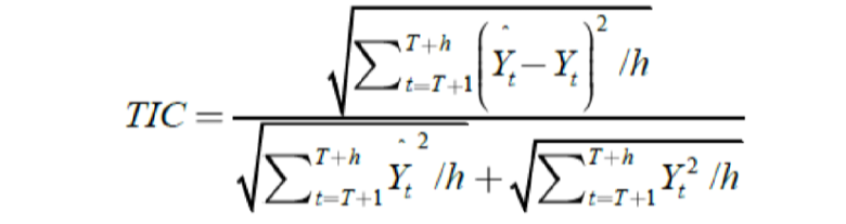
Where, Yt+1=Y; t this gives the value of the forecast variable in time “t” (Gujarati, 2012).

This study performs Jarque and Bera (1987) (JB) test for normality. We used this test to examine whether the residuals terms in the data are normally distributed. The JB test statistics formula is as under:

 

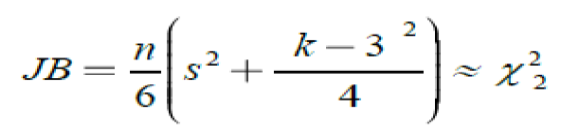
Where; k and n identifies as the regressors and observations respectively. The JB-test follows an asymptotic chi-squared distribution with two degrees of freedom. The skewness is a measure of the symmetric distribution of a data around its mean. The perfect symmetric data will have a skewness of zero. Kurtosis is a measure of the peakedness. For normal distribution kurtosis hold a value of 3. We examine how these two values are sufficiently different for zero and 3 respectively.

Next, we perform the Ljung-Box Q-test. Here the null hypothesis is that there is no autocorrelation up to order lags k, against the alternative hypothesis that some autocorrelation coefficient ρ(l), l = 1, ..., K, is non-zero. The equation of this tests is given by:

 

Where;

K, n and ρ(l) identifies the number of autocorrelation lags, observations and sample autocorrelation at lag l respectively. Nevertheless, assuming that the data is not accordance with the outcome of ARIMA estimation, then, on the basis of the null hypothesis, Q is distributed asymptotically with χ2 and degree of freedom is equal to the number of autocorrelations.

Results and Discussion

The descriptive statistics of both the series of guava area and production for the period 1997-98 to 2014-15 are provided in Table 1. The average value of the area was 61.62 thousand hectares ranging from 42.70 to 67.20. The standard deviation of guava area was reported 5.37. Similarly, the average value of guava production was 518.43 thousand tons. The minimum value was figured out 454.90 and maximum was 571.80 with a standard deviation of 32.12. Figure 1 presents the trend of variables in this study.

Moreover, Figure 2 presents the Correlogram of the original series of guava area. The series is stationary at a level as probability values of Q-statistics for all lags are insignificant. Additionally, the ACF (autocorrelation function) and PACF (partial autocorrelation function) spikes are limited to the bound area. Moreover, Figure 3 refers to the Correlogram for the original series of guava production. The production series is not stationary at a level as probability values of Q-statistic for all lags are significant, which concludes that the series is integrated. The non-stationary of guava production series is also determined by the spikes of ACF and PACF. It is visible in Figure 3 that all the spikes are not limited to the bound area of ACF and PACF, which reveals that the series is not stationary. Therefore, the series needs transformation to get a stationary series. Prior to check unit root both the series were transformed into logarithmic form. The issue of stationarity was handled by taking the difference. Results of the differenced series are provided in Figure 4. This shows that the production series is stationary at first difference as probability values of Q-statistic for all lags are insignificant. From the results of Figure 2 it clearly indicates that both ACF and PACF spikes patterns are all most close to zeros, which suggests that the series for guava area is pure white noise which means ARIMA (0,0,0) model is expected. Figure 4 shows that ACF patterns is the perfect reflection of damped sine wave or exponential decay while PACF pattern presents single positive spike at lag 1, which suggest ARIMA (1,1,0) model.

Table 1: Descriptive statistics of the series.

Parameters	Mean	Median	Max.	Min.	St. Dev.
Area	61.62	62.65	67.20	42.70	5.37
Production	518.43	518.90	571.80	454.90	32.12

Source: Author’s calculations.

To check the unit root test, this study used Augmented-Dickey Fuller (ADF) and Phillips-Perron (PP) test. Results of both the tests (ADF and PP) are provided in Table 2. These tests results show that guava area ~ I (0) while guava production ~ I(1).

Table 2: Results of unit root tests.

Parameter		ADF test	P value	PP test	P value	Conclusion
Area	Level	-3.24**	0.04**	-5.14	0.01**	I(0)
	Differenced	-	-	-	-
Production	Level	-2.36	0.38	-2.21	0.21	I(1)
	Differenced	-4.06	0.03**	-3.99	0.01**

Note: Asterisks shows significance level at **5%.

Source: Author’s calculations.

Generally, at this stage, various tentative models are estimated and different parameters are examined. The estimated models are compared with the given different criteria such as LogL, AIC, BIC and HQ. In both the cases of guava area and production series, the diagnostics of the nine alternative models are checked in order to choose the most appropriate models (Table 3). Furthermore, Table 3 shows that ARIMA (0,0,0) is the best model in the case of guava area series while ARIMA (1,1,0) in case of guava production series. The most appropriate model’s selections for both the series (guava area and production) were confirmed through ARIMA criteria of the graph (Figure 5 and 6). This criterion reveals that the best forecasted ARIMA models for guava area and production are (0,0,0) and (1,1,0) respectively in the case of Pakistan.

Many researchers have studied ARIMA model globally. Nevertheless, present literature is still deficient in this area of research. To the updated knowledge we

Table 3: ARIMA models fitted for time series data of guava area and production and corresponding selection criterion, i.e. AIC, BIC and HQ.

Parameter	Model	Log L	AIC	BIC*	HQ
Area	0,0,0	16.51	-1.61	-1.51	-1.60
	0,0,1	17.57	-1.62	-1.47	-1.59
	0,0,2	18.91	-1.65	-1.45	-1.63
	1,0,1	18.53	-1.61	-1.41	-1.58
	1,0,0	16.97	-1.55	-1.40	-1.53
	2,0,1	19.77	-1.64	-1.39	-1.60
	2,0,0	17.79	-1.53	-1.33	-1.50
	1,0,2	18.98	-1.55	-1.31	-1.51
	2,0,2	20.36	-1.59	-1.29	-1.55
Production	1,1,0	31.57	-3.17	-3.02	-3.15
	2,1,1	33.24	-3.13	-2.89	-3.10
	2,1,0	31.61	-3.07	-2.88	-3.04
	1,1,1	31.60	-3.06	-2.87	-3.03
	2,1,2	34.47	-3.16	-2.86	-3.12
	0,1,1	29.32	-2.93	-2.77	-2.91
	0,1,2	30.35	-2.92	-2.73	-2.90
	1,1,2	29.51	-2.72	-2.47	-2.68
	0,1,0	24.83	-2.53	-2.43	-2.52

Source: Author’s calculations.

believe that there is not a single study available based on guava area and production. In this area of research, the most similar study was found of Ullah et al. (2018) taking the case of Pakistani peach area and production. Their study revealed that ARIMA (1,1,0) was the most appropriate model for both peach area and production. This result is quite similar to the finding of our study. Similarly, Khan et al. (2008) used the ARIMA approach in the case of Pakistani mango production. The outcome of their study was ARIMA (1,1,1). Moreover, in the similar context Jam et al. (2013) forecasted the mango area using ARIMA model. The best forecasted was found ARIMA (0,1,0). Furthermore, using the ARIMA model Ahmad and Mustafa (2006) conducted study on Pakistani Kinnow production. The best forecasted was selected was ARIMA (3,1,2). Rahman and Baten (2016) have also used ARIMA model and study were conducted on Bangladesh black gram. The best forecasted and preferred model was found ARIMA (0,1,0). Moreover, Iqbal et al. (2005) found different ARIMA model for their respective study on Pakistan wheat area and production. The best model was ARIMA (1,1,1) and ARIMA (2,1,2).

The goodness of fit of the model is examined with the help of Ljung-Box Q-statistic. Figure 7 presents the Correlogram of guava area series after the determination of ARIMA (0,0,0) model. These results suggest that corresponding probability values of Q-Stat for all lags are insignificant, which means that residuals are not serially correlated and the best suitable ARIMA (0,0,0) model of guava area series is free from serial correlation. Similarly, Correlogram of guava production series after the determination of ARIMA (1,1,0) are presented in Figure 8. These results suggest that probability values of Q-stat for all lags are insignificant, which means that residuals are not auto correlated and the best appropriate ARIMA (1,1,0) model of guava production series is free from serial correlation.

The ARIMA model for guava was selected as ARIMA (0,0,0) and for production (1,1,0). The respective models quality, performance and predictability power was chosen using the lowest error’s values of RMSE, MAE, MAPE and TIC (Table 4). The model with minimum lowest error’s values is assumed to describe the data series adequately.

Table 4: Results of evaluating forecast measures.

Model	RMSE	MAE	MAPE	TIC
ARIMA (0,0,0)	5.22	3.14	5.77	0.04
ARIMA (1,1,0)	0.08	0.065	1.04	0.006

Source: Author’s calculations.

Figures 9 and 10 display histogram of the standardised residuals of normality test of the estimated models. Evidence of this test shows that among the residual no autocorrelation was detected for both area and production of guava at 5% level of significance. Furthermore, Jarque-Bera statistic (Table 5) shows that standardised residuals of both the series are normally distributed.

Table 5: Jarque-Bera test of residuals diagnostics.

Series	Skewness	Kurtosis	Jarque-Bera	Probability
Area	-0.42	4.70	2.71	0.26
Production	-0.41	2.71	0.53	0.77

Source: Author’s calculations.

Table 6: Forecasted area and production of guava in Pakistan.

Years	Area (000 hectares)	Production (000 tonnes)
2015-16	61.37	491.72
2016-17	61.37	493.85
2017-18	61.37	495.56
2018-19	61.37	496.94
2019-20	61.37	498.05
2020-21	61.37	498.95
2021-22	61.37	499.68
2022-23	61.37	500.26
2023-24	61.37	500.73
2024-25	61.37	501.11
2025-26	61.37	501.41
2026-27	61.37	501.66
2027-28	61.37	501.85
2028-29	61.37	502.01
2029-30	61.37	502.14.

Source: Author’s calculations.

Results of the best ARIMA model for guava area was concluded ARIMA (0,0,0) while the best forecasted model for guava production was estimated as ARIMA (1,1,0). The forecasted period was from 2015-2016 to 2029-2030. Forecasted area and production of guava are tabulated in Table 6. The projected area of guava for the forecasted period is 61.37 thousand hectares each year. The forecasted production of guava is 491.72 thousand tonnes in the year 2015-16. The forecasted production will increase to 502.14 thousand tonnes in the year 2029-30. The comparison trend of the original and forecasted guava area and production series are presented in Figure 11. This figure reveals that the guava area series has a static trend, while guava production series has an upward trend over the time span from 2015-2016 to 2029-2030.

Conclusions and Recommendations

In this study guava area and production of Pakistan has been forecasted, using the Box-Jenkins approach for the period 2015-16 to 2029-30. This approach concludes that appropriate models to forecast area and production of guava in Pakistan are ARIMA (0,0,0) and ARIMA (1,1,0), respectively. The projected area of guava for the forecasted period is 61.37 thousand hectares each year showing a static trend throughout the forecasted period. The forecasted production of guava is 502.14 thousand tonnes in the year 2029-30 showing 2.12% increasing trend in production during the forecasted period. The current situation of guava production is quite favourable; however, to increase more guava production using of improved guava cultivars, improved system of irrigation and adequate cultural practices should be adopted. A comprehensive strategy should be adopted to bring more barren land under guava cultivation. These approaches would help to increase guava production in the future.

Novelty Statement

Area and production forecasting plays an important role in planning, policy making and research in the modern world. ARIMA model was used to forecast the guava area and production of Pakistan. Findings of the study will be useful for research-ers, producers and policymakers.

Author’s Contribution

Dilawar Khan and Arif Ullah designed, analysed, and organised the manuscript. Ihsan Ullah drafted the paper. Zainab Bibi, Muhammad Zulfiqar and Zafir Ullah Khan helped in proof reading and edited the manuscript.

References

Ahmad, B., A. Ghafoor. A. and H. Badar. 2005. Forecasting and Growth Trends of Production and Export of Kinnow from Pakistan. J. Agric. Soc. Sci., 1(1): 20-24.

Ahmad, B. and K. Mustafa. 2006. Forecasting kinnow production in Pakistan : An econometric analysis. Int. J. Agric. Biol. 8(4): 455-458.

Amin, M., M. Amanullah and A. Akbar. 2014. Time series modelling for forecasting wheat production of Pakistan. J. Anim. Plant Sci. 24(5): 1444-1451.

Anderson, T.W. 1971. The statistical analysis of time series. John Wiley, New York.

Badmus, M.A. and O.S. Ariyo. 2011. Forecasting cultivated areas and production of maize in Nigerian using ARIMA Model. Asian J. Agric. Sci., 3(3): 171-176.

Boken, V.K. 2000. Forecasting spring wheat yield using time series analysis. Agron. J. 92(6): 1047-1053. https://doi.org/10.2134/agronj2000.9261047x

Box, G.E.P. 1976. Jenkins. Time series analysis: forecasting and control, Holdon–Day, San Francisco. USA.

Dickey, D.A. and W.A. Fuller. 1979. Distribution of the estimators for autoregressive time series with a unit root. J. Am. Stat. Assoc. 74: 427-431. https://doi.org/10.1080/01621459.1979.10482531

GoP. 2019. Agricultural statistics of Pakistan. Islamabad Econ. Div., Minist. Food, Agric. Livest., GoP.

GoP. 2015. Economic survey of Pakistan 2014–15. Islamabad: Minist. Finance, GoP, Fed. Secretariat.

GoP. 2016. Economic survey of Pakistan 2015–16. Islamabad: Minist. Finance, GoP, Fed. Secretariat.

Gujarati, D. 2012. Econometrics by example. Palgrave Macmillan, Macmillan Publishers Limited, UK.

Hyndman, R.J. 2006. Koehler A.B. Another look at measures of forecast accuracy. Int. J. Forecasting. 22(4): 679–688. https://doi.org/10.1016/j.ijforecast.2006.03.001

Iqbal, N., K. Bakhsh, A. Maqbool and A.S. Ahmad. 2005. Use of the ARIMA model for forecasting wheat area and production in Pakistan. J. Agric. Soc. Sci. 1(2):120-122.

Jam, F.A., S. Mehmood and Z. Ahmad. 2013. Time series model to forecast area of mangoes from Pakistan : An application of univariate ARIMA model. Acad. Contemp. Res. 2: 10–15.

Jambhulkar, N.N. 2013. Modeling of rice production in Punjab using ARIMA model. Int. J. Sci. Res. 2(8): 2-3. https://doi.org/10.15373/22778179/AUG2013/1

Jarque, C.M. and A.K. Bera. 1987. A test for normality of observations and regression residuals. Int. Stat. Rev. 55: 163–172. https://doi.org/10.2307/1403192

Khan, M., K. Mustafa, M. Shah, N. Khan and J.Z. Khan. 2008. Forecasting mango production in Pakistan an econometric model approach. Sarhad J. Agric. 24(2): 363-370.

Khushk, A.M., A. Memon and M.I. Lashari. 2009. Factors affecting in guava production in Pakistan. J. Agric. Res. 47(2): 201-210.

Ljung, G. and G. Box. 1979. On a measure of lack of fit in time series models. Biometrika. 66(2): 265-270. https://doi.org/10.1093/biomet/66.2.265

PHDEC. 2017. Pakistan horticulture development and export company. Minist. Commerce. http://www.phdec.org.pk/phs.php Accessed on, August 19, 2017.

Philips, P.C.B. and P. Perron. 1988. Testing for a unit root in time series regression. Biometrika. 75(2): 335-346. https://doi.org/10.1093/biomet/75.2.335

Pindyck, R., S. Daniel and L. Rubinfeld. 1991. Economic models and economic forecasts, 3rd ed. McGraw Hill Int. Editions (Econ. Survey) New York, USA.

Qureshi, M.N., M. Bilal, M.K. Ali and R.M. Ayyub. 2014. Modelling of citrus fruits production in Pakistan. Sci. Int. 26(2): 733–737.

Rahman, N.M.F. and M.A. Baten. 2016. Forecasting area and production of black gram pulse in Bangladesh using ARIMA models. Pak. J. Agric. Sci. 53(4): 759-765. https://doi.org/10.21162/PAKJAS/16.1892

Sabir, H.M. and S.H. Tahir. 2012. Supply and demand projection of wheat in Punjab for the year 2011-2012. Interdisciplin. J. Contemp. Res. Bus. 3(10): 800-808.

Saeed, N., A. Saeed, M. Zakria and T.M. Bajwa. 2000. Forecasting of wheat production in Pakistan using ARIMA models. Int. J. Agric. Biol. 2(4): 352-353.

Suleman, N. and S. Sarpong. 2012. Forecasting milled rice production in Ghana using Box-Jenkins approach. Int. J. Agric. Manage. Dev. 2(2): 79-84.

Ullah, A., D. Khan and S. Zheng. 2017. The determinants of technical efficiency of peach growers: Evidence from Khyber Pakhtunkhwa, Pakistan. Custose @gronegócio on line. 13: 4.

Ullah, A., D. Khan and S. Zheng. 2018. Forecasting of peach area and production wise econometric analysis. J. Anim. Plant Sci. 28(4):121-1127.

UN. 2011. World population prospects the 2010 revision: Volume I: Comprehensive tables. New York. Dep. Econ. Soc. Aff. Popul. Div., U. N.