Research Article

Demand for Fruit Quantity and Quality in Pakistan: A Comparison of Urban and Rural Households

Abbas Ullah Jan1, Muhammad Fayaz1*, Yousaf Hayat2, Dawood Jan3 and Ghaffar Ali3

1Department of Agricultural and Applied Economics, The University of Agriculture, Peshawar, Pakistan; 2Department of Maths, Stats and Computer Sciences, The University of Agriculture, Peshawar, Pakistan; 3Department of Agricultural and Applied Economics, The University of Agriculture, Peshawar, Pakistan.

Received | May 31, 2017; Accepted | October 23, 2017; Published | November 09, 2017

*Correspondence | Muhammad Fayaz, Department of Agricultural and Applied Economics, The University of Agriculture, Peshawar, Pakistan;

Email: mfayaz@aup.edu.pk

Citation | Jan, A.U., M. Fayaz, Y. Hayat, D. Jan and G. Ali. 2017. Demand for fruit quantity and quality in pakistan: a comparison of urban and rural households . Sarhad Journal of Agriculture, 33(4): 647-652.

DOI | http://dx.doi.org/10.17582/journal.sja/2017/33.4.647.652

Keywords | Engel curve, Log-Log-Inverse function, Quality elasticity, Fruits, Urban and rural households, Pakistan

Introduction

Quality is one of the most often used words relating to foods and food services that interact with consumers (Herbert, 2001). Cardello (1997) while defining food quality has emphasized mainly on consumers’ acceptability as an appropriate measure of quality and argues that quality is no more or less than product acceptability. United States Department of Agriculture (USDA) Marketing Workshop Report defines food quality as ‘the combination of attributes or characteristics of a product that have significance in determining the degree of acceptability of the product to a user (Gould, 1977). Food quality emphasizes mainly on the consumers perceptions and acceptability. Therefore consumer models of food quality are actually perceived quality models, because quality is viewed in terms of consumer perceptions rather than based on product characteristics (Parasuraman et al., 1985).

Empirical research on food quality was initiated during 1950s, with main work by Houthakker (1957) wherein he expressed that increases in food expenditure could be devoted to increase in the quantity of food consumed, increase in the quality of the diet, or more generally some combination of the two. Hicks and Johnson (1968) further explained that when incomes increase above subsistence level, individuals begin to include items of higher quality in the bundles of goods which they purchase. McCarthy (1981), in his study on ‘quality effect in consumer behavior’ in Pakistan, elaborated that “as income rises in most instances people spend a portion of increase on larger quantities but much of the increase goes on higher-priced varieties”.

With the exception of McCarthy (1981) and recently Jan et al. (2008 a, b; 2009) there has been no empirical research literature available on food quality in Pakistan. Keeping in view the ever increasing demand for quality food from domestic market and abroad there is a great need of quantitative and empirical research on food quality. Since quality is a large research area having multiple dimensions, therefore the present study is mainly focused on estimating and comparing the quantity, expenditure and quality elasticities of fruits for urban and rural households in Pakistan.

Matrials and Method

Expanding the concept of Houthakker (1957), Hicks and Johnson (1968) provided methodology to separate quality and quantity components of income elasticity which is explained as under:

Consider a particular expenditure on food, F. Let X be the quantity of food in F and Y be the quality of food in F. It is assumed that F is functionally related to X and Y.

F = g(X, Y)……….(1)

In addition, it is assumed that individuals’ consumption of food is a function of per capita income. With I denoting the per capita income, this function is specified in the equation (2) as;

F = h (I)………(2)

Taking the total differentials of equations (1) and (2) and setting them equal to each other gives, on a slight rearrangement of terms we get,

 

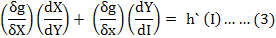
Where;

h`(I): Derivative of the equation (2) with respect to I, dX, dY; dI: Arbitrarily small changes in the noted variables; δg/δX and δg/δY: Partial derivatives of equation (1) with respect to X and Y respectively.

Multiplying both sides of equation (3) by I/F yields an expression for the income elasticity for food in terms of a weighted average of two terms as under:

 

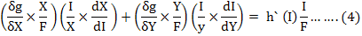
For sufficiently small changes in X, Y, and I, the two terms on the right-hand side of equation (4) can be interpreted as quantity and quality components of the income elasticity.

The first term in equation (4) is a product of two expressions which are rather easily interpretable. The term (δg/δX) (X/F), called a quantity weight, indicates how food expenditures change with the quantity of food consumed, and (I/X) (dX/dI) is a quantity elasticity. Together the two terms give the quantity component of the income elasticity. The second term can be interpreted similarly with respect to quality. The quantity component of the income elasticity decreases in relative importance as the level of income increases.

On the basis of pioneer work of Hicks and Johnson (1968), Gale and Huang (2007) proposed methodology to capture the effect of quality through a nonlinear Engel relationship. According to their model, Engel curve expresses the relationship between household expenditure and income, as given in equation (5).

e(Y) = pq(Y)……………..(5)

Equation (5) expresses that expenditure (e), which is a product of price (p) and quantity (q), depends upon income (Y). If prices are held constant, then elasticity of expenditure (e) with respect to Y becomes equal to that of quantity (q) with respect to income (Y); that is:

 

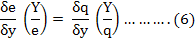
If cross sectional data is taken on consumption, expenditure, income and prices, then it can be assumed that prices do not change in the same year so relationship in equation (2) can practically be computed. Equation 6 suggests that if there is any increase in the expenditure that will be explicitly due to an increase in quantity consumed, and if any increase in price is observed that would then be because of the improvement in quality. Hence, to incorporate the effect of quality, equation (5) would transform, as follows:

e(Y) = v(Y)q(Y)……………(7)

Where;

v(Y): Variation in prices paid for quality.

Equation (7) can be reduced to equation (8) after taking its natural log and differentiating with respect to lny i.e.

 

The left-hand side of equation (8) represents expenditure elasticity (ε), while the first part of the right-hand side represents quality elasticity (θ) and the second part quantity elasticity (η); namely.

ε = θ + η ………..(9)

Equation (9) can be re-arranged to compute quality elasticity (θ), as follows.

θ = ε - η ………(10)

This methodology is similar to that of Hassan and Johnson (1977), who estimated elasticities of food consumption, expenditure and quality with respect to household income for Canadian households. At low income level when income (y) rises, the effect of income on consumption (q) is positive (δq/δy > 0), with the second derivative negative (δ2q/δ2y <0), suggesting that at sufficiently low income level almost all goods are normal. While with the further increase in income, δq/δy drops and at some level reaches zero; so in practice, Engel curve is not linear but nonlinear. Thus to capture nonlinear relationship of consumption (q) and income (Y), the log-log-inverse (LLI) form of Engel equation can be used.

lnq = α + βq(1/Y) + γqlnY + μ ………..(11)

where;

μ: Random error.

Similarly, for expenditure (e) and income (Y) relationship, equation (11) can be modified as:

lne = α + βe(1/Y) + γelnY + μ ………. (12)

Estimation of equations (11) and (12) would give values of parameters α, β, γ and if β is equal to zero, the LLI model would simplify to double log model, suggesting constant elasticities. Similarly, if γ is equal to zero, LLI model would simplify to log inverse model. However, if both β and γ are not equal to zero, then elasticities would be worked out, as follows:

η = - βq(1/Y) + γq …………(13)

ε = - βe(1/Y) + γe…………..(14)

Substituting values of η and ε from equations (13) and (14) into Equation (9) and (10), the quality elasticity (θ) would be computed.

In the above methodology there are mainly two equations (equations 11 and 12) that require data on fruit consumption, expenditure and income of the households which was obtained from household income and expenditure data of PLSM survey 2005, collected by Federal Bureau of Statistics, Government of Pakistan (GoP, 2005). This data includes 4342 urban and 5641 rural households from the four provinces of Pakistan (Islamabad Capital Territory excluded) whose data of fruit consumption, expenditure and income was available. As the collected data is cross sectional, therefore, the problem of hetroscedascity is suspected and is checked by using the Koenker-Basset (KB) test (Koneker and Basset, 1982). Autocorrelation is not considered a problem as the data is cross sectional (Hussain, 1991). Chow test (Chow, 1960) is used for structural differences in the consumption and expenditure models across the urban and rural households. As the sample size is reasonably large, therefore, the normality assumption can be relaxed (Gujarati, 2003) and the t and F tests can be used with confidence for hypothesis testing. The data is analyzed using SHAZAM (version 10) and SPSS (version 12) software.

Results and Discussion

The significance of the chow test suggests that there

Table 1: Empirical results of quantity elasticity model (equation 11).

Particulars	Urban	F-ratio	R2
All fruits	lnq = 2.522 + 849.434 (1/Y) + 0.664 lnY (18.7)* (7.2)* (50.1)*	3378.8*	0.61
Apple	lnq = 3.588 + 808.711(1/Y) + 0.492 lnY (25.6)* (5.8)* (36.3)*	1823.3*	0.56
Banana	lnq = - 0.339 + 327.225 (1/Y) + 0.456 lnY (-2.9)* (3.25)* (40.4)*	2386.1*	0.55
Citrus	lnq = 3.463 + 903.731(1/Y) + 0.538 lnY (19.3)* (6.2)* (30.4)*	924.3*	0.53
Dates	lnq = 4.869 – 204.072 (1/Y) + 0.307 lnY (19.8)* (-0.99) (12.7)*	278.7*	0.38
Grapes	lnq = 5.007 + 12.104 (1/Y) + 0.196 lnY (13.1)* (-0.03) (8.2)*	136.8*	0.42
Guava	lnq = 5.362 + 227.971 (1/Y) + 0.307 lnY (34.7)* (1.6) (20.3)*	557.3*	0.37
Mango	lnq = 3.468 + 586.6 (1/Y) + 0.543 lnY (3.2)* (0.6) (5.2)*	59.5*	0.54
	Rural
All fruits	lnq = 1.863 + 1116.052 (1/Y) + 0.736 lnY (12.7)* (12.7)* (49.1)*	3261.1*	0.54
Apple	lnq = 3.382 + 792.273 (1/Y) + 0.518 lnY (21.9)* (8.1)* (32.9)*	1409.1*	0.49
Banana	lnq = - 1.342 + 817.486 (1/Y) + 0.561 lnY (-10.5)* (10.5)* (43.1)*	2447.1*	0.51
Citrus	lnq = 3.962 + 646.044 (1/Y) + 0.488 lnY (19.2)* (5.2)* (23.1)*	741.1*	0.42
Dates	lnq = 4.856 – 162.977 (1/Y) + 0.310 lnY (15.7)* (-0.85) (9.8)*	278.5*	0.35
Grapes	lnq = 6.801 – 2072.989 (1/Y) + 0.134 lnY (9.9)* (-4.8)* (1.9)*	123.8*	0.55
Guava	lnq = 4.27 + 541.258 (1/y) + 0.427 lnY (26.5)*(5.6)* (25.8)*	874.7*	0.42
Mango	lnq = - 0.29 + 3324.238 (1/Y) + 0.929 lnY (-0.2) (4.0)* (6.9)*	55.4*	0.39

(Figures in parenthesis represent t-ratios and * represents significance at 5% level of significance)

 

Table 2: Empirical results of expenditure elasticity model (equation 12).

Particulars	Urban	F-ratio	R2
All fruits	lne = - 2.719 + 1129.828 (1/Y) + 0.818 lnY (-19.5)* (9.3)* (59.9)*	4727.7*	0.68
Apple	lne = - 1.851 + 1384.479 (1/Y) + 0.681 lnY (-12.3)* (9.2)* (46.7)*	2808.5*	0.66
Banana	lne = - 0.965 + 562.497 (1/Y) + 0.566 lnY (-8.1)* (5.4)* (48.7)*	3288.1*	0.63
Citrus	lne = - 1.173 + 952.461 (1/Y) + 0.602 lnY (-6.5)* (6.5)* (33.9)*	1174.8*	0.59
Dates	lne = 1.226 – 420.822 (1/Y) + 0.347 lnY (5.2)* (-2.1)* (15.1)*	436.8*	0.49
Grapes	lne = 2.156 – 1452.138 (1/Y) + 285 lnY (5.8)* (-3.4)* (8.1)*	255.5*	0.58
Guava	lne = 0.115 + 397.077 (1/Y) + 0.431 lnY (0.7) (2.8)* (27.7)*	1002.3*	0.51
Mango	lne = 0.126 + 47.312 (1/Y) + 0.518 lnY (0.1) (0.04) (4.8)*	61.2*	0.54
	Rural
All fruits	lne = - 2.961 + 1237.882 (1/Y) + 0.846 lnY (-19.3)* (13.4)* (53.7)*	3978.5*	0.58
Apple	lne = - 1.647 + 1218.336 (1/Y) + 0.667 lnY (-9.8)* (11.5)* (39.1)*	1810.4*	0.55
Banana	lne = - 1.774 + 947.789 (1/Y) + 0.652 lnY (-13.5)* (11.8)* (41.8)*	3090.3*	0.57
Citrus	lne = - 0.696 + 642.252 (1/Y) + 0.557 lnY (-3.2)* (4.9)* (24.9)*	916.1*	0.47
Dates	lne = 1.272 – 475.819 (1/Y) + 0.345 lnY (3.9)* (2.3)* (10.3)*	390.5*	0.43
Grapes	lne = 1.656 – 1783.874 (1/Y) + 0.345 lnY (2.3)* (-3.9)* (4.6)*	197.4*	0.66
Guava	lne = - 0.511 + 571.59 (1/Y) + 0.5 lnY (-3.1)* (5.8)* (29.3)*	1170.6*	0.49
Mango	lne = - 4.986 + 3429.95 (1/Y) + 1.038 lnY (-3.9)* (4.2)* (7.9)*	82.1*	0.49

(Figures in parenthesis represent t-ratios and * represents significance at 5% level of significance)

 

exist highly significant structural changes in the consumption and expenditure models of the urban and rural households therefore equations (11) and (12) are estimated separately. Regression results for quantity Engel equations and expenditure equations are reported in Table 1. The log-log-inverse model fits the data well, as both the βq and γq parameters are statistically significant in most equations. The highly significant F values indicate overall goodness of models. The R2 is quite reasonable for cross sectional data (World Bank, 2005). Based upon the results of K-B test there seems no hetroscedasticity in all the models.

Quantity elasticities

The estimate of the βq parameter is significantly different from zero in all equations estimated for rural and some for urban households, indicating that the income elasticity of demand depends on the level of household income. The βq estimate is not significantly different from zero for dates, grapes, guava and mango for urban households and dates for rural households suggesting constant income elasticity in case of these fruits. The sign of the estimate of βq indicates that the elasticity tends to increase as income rises in all fruits except grapes for rural households where it tends to decrease. Quantity-income elasticities of fruits (Table 3) are less than 1 for all fruits but not close to zero for both urban and rural households suggesting that households have not approached saturation levels of quantity consumed at the prevailing income level. Compared to rural households, quantity elasticities of all fruits, apple and citrus are high for urban household while that of the rest of fruits are high for rural households. Thus consumption of all fruits, apple and citrus is more sensitive to household income in urban areas and that of the rest of fruits show high income sensitivity in rural areas.

Expenditure elasticities

The estimated expenditure equations for both the urban and rural households are reported in Table 2. The parameter βe was statistically significant in almost all equations indicating that the expenditure elasticity varies with income for most of fruits. The only exception is mango where βe is not statistically significant (p > 0.05) suggesting constant expenditure elasticity for urban households. All expenditure elasticities (Table 3) are larger in magnitude than the corresponding quantity elasticities, reflecting a “quality” effect whereby expenditures on fruits rise faster than the quantity purchased when household income grows. The magnitude of the expenditure elasticities follows almost the pattern of quantity elasticities in terms of urban and rural households.

Quality elasticities

Quality elasticities are positive (Table 3) for all the individual fruits and all fruits as a group for both the urban and rural households indicating a quality effect. The positive quality elasticities suggest that both the urban and rural households purchase higher quality fruits as their income increases and are willing to pay a higher price for enhanced quality. The urban households are more responsive to quality than those in the rural areas in all fruits as a group and apple, banana, and grapes individually. Quality response is more in dates, mango and particularly guava for rural households. In case of citrus quality response is almost the same for urban and rural households.

The estimates of quantity, expenditure and quality elasticities obtained for all the fruits in this study indicating a greater similarity to the estimates of Gale and Haung (2007), Tey et al. (2008; 2009), Jan et al. (2008a; 2008b; 2009), Ogundari (2012) and Fayaz et al. (2014; 2016) obtained for other food products in their studies.

Conclusion and Recommendations

The results of this study provides sufficient evidence that generally in Pakistan, fruit consumption with respect to income shows a nonlinear trend rather than a linear one and LLI formulation of Engel curve can best capture such behavior. With the increase in income households in Pakistan purchase higher quality fruits at higher price. Comparatively urban households are more responsive to quality than those in the rural areas in all fruits as a group and apple, banana

Table 3: Quantity, expenditure and quality elasticity (Urban and Rural).

Particulars	Quantity Elasticity (η)		Expenditure Elasticity (ε)		Quality Elasticity (θ)
	Urban	Rural	Urban	Rural	Urban	Rural
All Fruits	0.6098	0.6091	0.7459	0.7053	0.1361	0.0961
Apple	0.4534	0.4377	0.6047	0.5435	0.1512	0.1058
Banana	0.4355	0.4702	0.5307	0.5467	0.0952	0.0765
Citrus	0.4829	0.4173	0.5439	0.4867	0.0610	0.0694
Dates	0.3186	0.3289	0.3708	0.4000	0.0523	0.0712
Guava	0.2965	0.3417	0.3397	0.5238	0.0431	0.1820
Grapes	0.2939	0.3695	0.4082	0.4393	0.1143	0.0698
Mango	0.5103	0.5247	0.5154	0.6208	0.0051	0.0961

and grapes individually. Quality response is high in dates, mango and particularly in guava for rural households. It is concluded that there exists greater potential of increased profits for entrepreneurs involved in the production and marketing of fruits if they focus on quality enhancement as both the urban and rural households are willing to pay a higher price for higher quality fruits. However further research is needed to find out those quality attributes of fruits that are perceived appealing by consumers so that firms engaged ensuring fruit quality can concentrate on them to provide the desired quality in line with the consumers’ specification .

Authors’ Contribution

This study is a collaborative effort of all authors. First and second authors designed the study, performed statistical analysis and drafted the manuscript. Third and fourth authors provided technical guidance, supervision and checked the work. Last author supported in data collection, data entry and analysis.

References

Cardello, A.V. 1995. Food Quality: Relativity, Context and Consumer Expectations. Food Quality and Preference. 6(3): 163–70.

Cardello, A.V. 1997. Perceptions of Food Quality. In Food Storage Stability by I. R. Taub and R.P. Singh. CRC Press, Boca Raton Florida: 1-37.

Chow, G.C. 1960. Tests of equality between sets of coefficients in two linear regressions. Econometrica. 28(3): 591-605.

Fayaz, M., Jan, A.U. and Jan, D. 2014. Quality elasticity of vegetable consumption in Pakistan: a comparison of urban and rural households. Sarhad J. Agric. 30(4): 451-458.

Fayaz, M., A. Jan, D. Jan, G. Ali and Y. Hayat. 2016. Does the quantity and quality of cereal respond to changes in income? Evidence from Pakistan. Sarhad J. Agric. 32(3): 177-183.

Gale, F. and K. Huang. 2007. Demand for food quantity and quality in China. U.S. Department of Agriculture. Econ. Res. Service. ERR-32. Washington D.C.

GoP. 2005. Pakistan Social and Living Standards Measurement Survey. Federal Bureau of Statistics. Government of Pakistan, Islamabad.

Gould, W.A. 1977. Food Quality Assurance. AVI Publishing, Westport.

Gujarati, D.N. 2003. Basic Econometrics, 4th edition, McGraw-Hill Inc. NY, USA. p.110.

Hassan, Z.A. and S.R. Johnson. 1977. Urban food consumption patterns in Canada: An empirical analysis. Agriculture Canada Publication No.77/1.

Herbert, L.M. 2001. Criteria of food quality in different contexts. Food Service Technol. 1 (2): 67–77.

Hicks, W. W. and S.R. Johnson. 1968. Quantity and quality components for income elasticities of demand for food. Am. J. Agric. Econ. 50:1512-1517.

Houthakker, H.S. 1957. An international comparison of household expenditure patterns. Econometrica. 25:532-551.

Hussain, A. 1991. Resource Use, efficiency and returns to scale in Pakistan: a case study of Peshawar Valley. Staff paper series. Deptt. Of Agric. and Applied Economics, University Of Minnesota.

Jan, A., A. F. Chishti, D. Jan and M. Khan. 2008a. Estimating consumers’ response to food quality: A case of Pakistan fruits. Sarhad J. Agric. 24(1): 151-154.

Jan, A., A.F. Chishti, D. Jan and M. Khan. 2008b. Milk Quality in Pakistan: Do Consumers Care? Sarhad J. Agric. 24 (2): 168-171.

Jan, A, D. Jan, G. Ali, M. Fayaz and M. Khan. 2009. Consumers’s response to milk quality: A comparison of urban and rural Pakistan. Sarhad J.Agric. 25 (2).

Koenker, R. and G. Basset. 1982. Robust test of hetroscedasticity based on regression quantiles. Econometrica. 50: 43-61. https://doi.org/10.2307/1912528

McCarthy, F.D. 1981. Quality effects in consumer behavior. Pak. Dev. Rev. 2(20): 133-150.

Tey, Y. S., F.M. Arshad, M. N. Shamsudin, Z. Mohamed and A. Radam. 2008. Demand for meat quantity and quality in Malaysia: Implications to Australia. MPRA Paper No. 15032. Available at: http://mpra.ub.uni-muenchen.de/15032/.

Tey, Y. S., M. Nasir, S., Zainalabidin, M., Jinap, S. and A. Gariff, R. 2009. Demand for quality vegetables in Malaysia. Int. Food Res. J. 16:313-327.

Parasuraman, A., V.A. Zeithaml and L. Berry. 1985. A conceptual model of service quality and its implications for future research. J. Mark. 49: 41–50. https://doi.org/10.2307/1251430

World Bank. 2005. Introduction to poverty analysis. World Bank Instt., Washington DC: 13 www.businessdictionery.com, last visited on May 2, 2009. http://en.wikipedia.org/wiki/Quality, last visited on May 2, 2009.

Ogundari, K. 2012. Demand for quantity versus quality in beef, chicken and fish consumption in Nigeria, Department of Food Economics and Consumption Studies, University of Kiel, Kiel,Germany.