Research Article

ANOVA or MANOVA for Correlated Traits in Agricultural Experiments

Iftikhar ud Din* and Yousaf Hayat

Department of Statistics, The University of Agriculture, Peshawar, Khyber Pakhtunkhwa, Pakistan.

Received | December 02, 2020; Accepted | April 03, 2021; Published | September 03, 2021

*Correspondence | Iftikhar-ud-Din, Department of Statistics, The University of Agriculture, Peshawar, Khyber Pakhtunkhwa, Pakistan; Email: iftikhar.din1@gmail.com

Citation | Din, I. and Y. Hayat. 2021. ANOVA or MANOVA for correlated traits in agricultural experiments. Sarhad Journal of Agriculture, 37(4): 1250-1259.

DOI | https://dx.doi.org/10.17582/journal.sja/2021/37.4.1250.1259

Keywords | Analysis of variance, Multivariate analysis of variance, Agricultural experiments, Dependent traits

Introduction

Analysis of variance (ANOVA) play a vital role in analyzing the data to compare the average effect of more than two treatments. It can be applied to varieties of problems relating to the disciplines like agriculture, biology, biotechnology, medical, climate change, engineering, economics, business industry and researches of many other sciences (Frost, 2020). In specific, agricultural experiments involving different treatments and/or factors which are compared under various experimental conditions, is not possible without the use of ANOVA model. ANOVA partitions the total variation in to components of variation and has the capability to compare the treatment means simultaneously by applying a single F-test (Steel et al., 2008).

In agricultural trials, an experiment is conducted by using an appropriate experimental design and the data is collected regarding more than one traits and analyzed by applying independent ANOVA for each of the trait recorded (Montgomery, 2013).

One by one, to investigate the effect of different factors or various levels of a single factor involved, we hypothesized that it will influence the response variable which can be a yield, number of tillers per plant, root length, leaf area, plant height etc., the motive is to test whether significance difference among the levels of a single factor exist (Kothari, 1985).

The ANOVA in which a single factor (having more than two levels) is investigated, called one-way classification and is called two-way classification when two factors are investigated at the same time (Gomez and Gomez, 1984).

ANOVA works well when the interest lies to compare the average effect of different treatments/verities by considering only a trait/response variable. However, in most of the agricultural experiments the response variables/traits are not independent at all because of having logical significant interactions, which in result compile the error substantially (Bray and Maxwell, 1985).

In a situation where, multiple inter-correlated traits are involved in the experiment, which is often the case with agricultural experiments, the most appropriate technique for analyzing the data is multivariate analysis of variance (MANOVA) instead of ANOVA (Oehlert, 2000).

MANOVA is the simple extension of ANOVA by considering multiple responses to investigate the mean differences instead of assessing the single response variable. The MANOVA provides additional information regarding the statistical model when the multiple response variables are correlated. It provides greater statistical power in case of correlated traits, evaluate pattern among the multiple correlated traits and it maintains the joint error rate, which is not possible by using ANOVA (Porter and Orailly, 2017). The MANOVA can usefully be employed for the experimental situations where the experiment is conducted for several years/seasons and/or multiple locations with same type of treatments and randomized layout.

MANOVA model is implied under the assumptions that the observations are sampled from the population and their selection is randomly made and independently. Further, each dependent variable must be continuous and within each group of categorical independent variables these dependent variables follow a multivariate normal distribution (Brito and Duarte, 2012).

The MANOVA model

Consider an experiment carried in randomized complete block design having r replications for comparing v treatments on p-variables (Parsad et al., 1987). Let the observation of the kth response variable for the ith treatment in the jth replication is represented by Yijk, where, I = 1,2,…, v; j = 1,2,…, r; k =1,2,…, p.

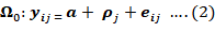
Then the ‘a’ two way classified multivariate model Ω can be represented by,

Here; μ= μ1+ μ2+….. μp is the p ×1 vector of general means, τi = (ti1 ti2 ….tip) indicate the ith treatment effects on p-characters (traits), and ρj = (rj1 rj2 ….rjp) denote the jth replication effect on p-characters. eij = (eij eij ….eijp) is a p ×1 random vector associated with Yijk having p variate normal distribution) Np (0, Σ).

The null hypothesis is whether significant difference between treatment exist i.e. H0: (ti1 ti2 ….tip) = (t1 t2 ….tp) (say) for i = 1, 2, …, p against the alternative H1= at least two of the treatment effects are significantly different. Assuming H0 is true, the model (1) reduces to:

Where;

Test statistics for MANOVA

In order to test the significance of the effects in the MANOVA table the following test statistics are more common:

Wilks lambda: Let H denote the sum of squares and sum of cross product matrices of treatments, E indicate the sum of squares and cross products relating to error and T denote the subsequent quantities for the totals.

Wilks Lambda is the ratio of the determinant of the error sums of squares and cross products matrix E to the determinant of the total sum of squares and cross products matrix T= H + E. That is:

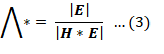
The null hypothesis of equality of treatment mean vectors is rejected if the ratio of generalized variance (Wilk’s lambda statistic) Λ* is too small i.e. H is large relative to E. Pillai Trace: It is formulated by multiplying H by the inverse of the total sum of squares and cross products matrix T = H + E. Large value of the test statistics means H is relatively large to E, which leads to the rejection of the null hypothesis.

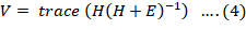
Hotelling-lawley trace: To obtain test statistics for Hotelling Trace, the inverse of E is multiplied by H (sum of squares and sum of cross product matrices of treatments) and the trace of the resultant matrix is taken. For Larger H in comparison to E, means large value of the test statistics, large value of Hotelling-Lawley trace, leads to the rejection of the null hypothesis.

Roy’s maximum root: Here, H is multiplied by the inverse of E, and from the result and matrix the largest eigen value is obtained. Roy’s root will be large if H is substantially large compare to E, which leads to the rejection of the null hypothesis.

Largest eigenvalue of HE-1: Each of the above test statistics has approximately F distribution, consequently, make use of tables for F test statistics is permissible. Keeping in view the use of appropriate statistical method for multiple correlated traits in agricultural experiments, the present research study was conducted to compare the results of ANOVA and MANOVA by considering simulated data obtained for a completely randomized design (CRD).

Parsad et al. (2004) considered the height of plant and the number of tillers per plant and measured the growth after six weeks of their transplantation. It was observed that taller the plant and greater the number of tillers per plant, higher will be the rice yield.

Materials and Methods

Numerous real world problems demand the use of appropriate multivariate analysis of variance (MANOVA). In many agricultural experiments, generally the data on more than one character is observed. One common example is grain yield and straw yield. The other characters on which the data is generally observed are the plant height, number of green leaves, germination count, etc. However, the comparative study of MANOVA and ANOVA require the data regarding the dependent variables having specific correlation coefficient. To investigate varying conditions of the traits in MANOVA and the corresponding ANOVA, simulated data is considered to illustrate the comparison. For simulations and modeling fitting SPSS version 26 is used.

We consider two correlated parameters which are yield (kg/hectare) and plant height (cm). Initially, parameters data are set for low correlation coefficient (r= 0.055) between the yield and plant height was considered. Further, the related three independents (factors) are incorporated against two correlated parameters. They are 2 levels of irrigation, 2 varieties and 5 nitrogen levels. Consequently, the model becomes 2×2×5 multivariate factorial experiment in CRD. For the stated model, MANOVA and ANOVA techniques were incorporated and the significance status of the effects were judged from the corresponding p-values.

The above set of independent variables are maintained to simulate second set of data but moderate correlation coefficient (r= 0.55) is maintained between the two dependent variables. The corresponding fitted models were analyzed to check the behavior of the main effects and interactions in the change environment of MANOVA as compared to ANOVA. The significance status and relative change in the p-values are the criterion used to discriminate between the two models.

The above mentioned procedure is repeated by inducing strong correlation coefficient (r= 0.8) between the two dependent variables and the estimates are reassessed. Based on the results of the corresponding ANOVA and MANOVA models, valid conclusion regarding the shift from MANOVA to ANOVA is established, and significance of various effects of the factors and their interactions are decided by their corresponding p-value

Results and Discussion

To illustrate the comparative analysis between MANOVA and ANOVA models, two dependent variables having small Pearson correlation coefficient are simulated and the output between these two competing models are compared. The linear relationship between the dependent variables is gradually increased and said comparison is reassessed.

Case 1: The analysis started by simulating two dependent variables having small Pearson correlation coefficient (r = 0.055) along with three related independent variables. Table 1 shows MANOVA for two dependent variables having low correlation coefficient (r= 0.055). It is evident from all the multivariate tests (Pillai trace, Wilks Lanbda, Hotelling’s trace, and Roy’s largest root) that the main effects and interactions with the exception of irrigation × varieties (I×V) possess highly significant effect on the joint dependent variables of yield and plant height.

 

Table 1: MANOVA for two very low correlated dependent variables (r =0.055).

Multivariate testsa
Effect		Value	F	Hypothesis df	Error df	Sig.
Irrigation (I)	Pillai's Trace	0.700	22.178	2	19	0.000
	Wilks' Lambda	0.300	22.178	2	19	0.000
	Hotelling's Trace	2.335	22.178	2	19	0.000
	Roy's Largest Root	2.335	22.178	2	19	0.000
Varieties (V)	Pillai's Trace	0.995	1737.319	2	19	0.000
	Wilks' Lambda	0.005	1737.319	2	19	0.000
	Hotelling's Trace	182.876	1737.319	2	19	0.000
	Roy's Largest Root	182.876	1737.319	2	19	0.000
Nitrogen (N)	Pillai's Trace	1.055	5.582	8	40	0.000
	Wilks' Lambda	0.014	35.075	8	38	0.000
	Hotelling's Trace	64.432	144.972	8	36	0.000
	Roy's Largest Root	64.356	321.781	4	20	0.000
I * V	Pillai's Trace	0.063	0.636	2	19	0.540
	Wilks' Lambda	0.937	0.636	2	19	0.540
	Hotelling's Trace	0.067	0.636	2	19	0.540
	Roy's Largest Root	0.067	0.636	2	19	0.540
I * N	Pillai's Trace	1.058	5.618	8	40	0.000
	Wilks' Lambda	0.022	27.281	8	38	0.000
	Hotelling's Trace	40.826	91.858	8	36	0.000
	Roy's Largest Root	40.736	203.681	4	20	0.000
V * N	Pillai's Trace	1.085	5.929	8	40	0.000
	Wilks' Lambda	0.034	21.064	8	38	0.000
	Hotelling's Trace	25.024	56.303	8	36	0.000
	Roy's Largest Root	24.882	124.412	4	20	0.000
I * V * N	Pillai's Trace	0.994	4.945	8	40	0.000
	Wilks' Lambda	0.035	20.467	8	38	0.000
	Hotelling's Trace	26.341	59.267	8	36	0.000
	Roy's Largest Root	26.309	131.544	4	20	.000

 

Table 2: Univariate ANOVA for each dependent variable (yield and plant height).

Tests of between-subjects effects
Source	Dependent variable	Type III sum of squares	df	Mean square	F	Sig.
Model	Yield	3440012.500a	20	172000.625	2274.388	0.000
	Plant height	1605563.871b	20	80278.194	4175.639	0.000
Irrigation (I)	Yield	3515.625	1	3515.625	46.488	0.000
	Plant height	1.088	1	1.088	0.057	0.814
Varieties (V)	Yield	276390.625	1	276390.625	3654.752	0.000
	Plant height	.926	1	.926	0.048	0.828
Nitrogen (N)	Yield	97022.500	4	24255.625	320.736	0.000
	Plant height	45.706	4	11.427	0.594	0.671
I * V	Yield	.625	1	.625	0.008	0.928
	Plant height	25.426	1	25.426	1.323	0.264
I * N	Yield	61612.500	4	15403.125	203.678	0.000
	Plant height	46.039	4	11.510	0.599	0.668
V * N	Yield	37587.500	4	9396.875	124.256	0.000
	Plant height	54.440	4	13.610	0.708	0.596
I * V * N	Yield	39777.500	4	9944.375	131.496	0.000
	Plant height	37.832	4	9.458	0.492	0.742
Error	Yield	1512.500	20	75.625
	Plant height	384.507	20	19.225
Total	Yield	3441525.000	40
	Plant height	1605948.378	40

 

Table 3: MANOVA for two low correlated dependent variables (r =0.19).

Multivariate testsa
Effect		Value	F	Hypothesis df	Error df	Sig.
Irrigation (I)	Pillai's Trace	0.710	23.285	2	19	0.000
	Wilks' Lambda	0.290	23.285	2	19	0.000
	Hotelling's Trace	2.451	23.285	2	19	0.000
	Roy's Largest Root	2.451	23.285	2	19	0.000
Varieties (V)	Pillai's Trace	0.995	1736.571	2	19	0.000
	Wilks' Lambda	0.005	1736.571	2	19	0.000
	Hotelling's Trace	182.797	1736.571	2	19	0.000
	Roy's Largest Root	182.797	1736.571	2	19	0.000
Nitrogen (N)	Pillai's Trace	1.088	5.96	8	40	0.000
	Wilks' Lambda	0.014	35.749	8	38	0.000
	Hotelling's Trace	64.279	144.628	8	36	0.000
	Roy's Largest Root	64.164	320.818	4	20	0.000
I * V	Pillai's Trace	0.263	3.382	2	19	0.055
	Wilks' Lambda	0.737	3.382	2	19	0.055
	Hotelling's Trace	0.356	3.382	2	19	0.055
	Roy's Largest Root	0.356	3.382	2	19	0.055
I * N	Pillai's Trace	1.001	5.007	8	40	0.000
	Wilks' Lambda	0.023	26.348	8	38	0.000
	Hotelling's Trace	40.834	91.876	8	36	0.000
	Roy's Largest Root	40.809	204.043	4	20	0.000
V * N	Pillai's Trace	1.164	6.960	8	40	0.000
	Wilks' Lambda	0.031	22.309	8	38	0.000
	Hotelling's Trace	25.133	56.549	8	36	0.000
	Roy's Largest Root	24.879	124.395	4	20	0.000
I * V * N	Pillai's Trace	1.009	5.089	8	40	0.000
	Wilks' Lambda	0.035	20.660	8	38	0.000
	Hotelling's Trace	26.363	59.316	8	36	0.000
	Roy's Largest Root	26.315	131.575	4	20	0.000

 

The corresponding univariate ANOVA carried out separately for each dependent variable yield and plant height reveals a different look as compared to MANOVA. The detail analysis given in Table 2 shows that interaction of irrigation × varieties as before is non-significantly effecting yield as well as plant height separately, the same is the case in MANOVA. However, apart from irrigation × varieties interaction all the remaining main effect and interactions possess highly significant effect on the yield but insignificantly effecting the other dependent variable plant height. These results clearly demonstrate that when the two traits are correlated (even low correlation coefficient), the results of ANOVA will be misleading in terms of investigating the main effects as well as interaction between/among the independent factors involved in the model.

Case 2: In the second case, a low to moderate correlation coefficient (r = 0.187) between the plant height and yield is considered and the results of MANOVA and ANOVA are displayed in Tables 3 and 4, respectively. From Table 3, it is evident that after applying 2×2×5 factorial MANOVA, the listed multivariate tests shows that all the main effects and their interactions are affecting the joint dependent variables with high significance apart from irrigation×varieties (I×V) interaction. On the other hand, its counterpart ANOVA (Table 4) is providing totally different results, it shows that all the main effects and their interactions have insignificant effect on the plant height except irrigation × varieties (I×V) interaction. The results of MANOVA in comparison to ANOVA, suggests that correlated traits can affect the significance of the main effects and their interactions.

Case 3: The above discussion is extended to the situation where moderate correlation exist among the dependent variables (r= 0.55, p <.001). Table 5 shows that for the simulated data of the two dependent variables all the main effects and interactions are highly significant (p <0.001) except for the interaction of irrigation × varieties, which shows insignificant effect on the joint dependent variable in the MANOVA model.

The corresponding between subjects ANOVA (Table 6) gives a different picture. The interaction is still insignificant for both the parameters. Main effect

 

Table 4: Univariate ANOVA for each dependent variable separately.

Tests of between-subjects effects
Source	Dependent Variable	Type III Sum of Squares	df	Mean Square	F	Sig.
Model	Yield	3440012.500	20	172000.625	2274.388	0.000
	Plant Height	2740180.131	20	137009.007	4.509	0.001
Irrigation (I)	Yield	3515.625	1	3515.625	46.488	0.000
	Plant Height	78307.356	1	78307.356	2.577	0.124
Varieties (V)	Yield	276390.625	1	276390.625	3654.752	0.000
	Plant Height	44579.859	1	44579.859	1.467	0.240
Nitrogen (N)	Yield	97022.500	4	24255.625	320.736	0.000
	Plant Height	77925.456	4	19481.364	0.641	0.639
I * V	Yield	0.625	1	0.625	0.008	0.928
	Plant Height	216115.156	1	216115.156	7.112	0.015
I * N	Yield	61612.500	4	15403.125	203.678	0.000
	Plant Height	64102.499	4	16025.625	0.527	0.717
V * N	Yield	37587.500	4	9396.875	124.256	0.000
	Plant Height	169210.340	4	42302.585	1.392	0.273
I * V * N	Yield	39777.500	4	9944.375	131.496	0.000
	Plant Height	40278.189	4	10069.547	0.331	0.854
Error	Yield	1512.500	20	75.625
	Plant Height	607740.169	20	30387.008
Total	Yield	3441525.000	40
	Plant Height	3347920.300	40

 

Table 5: MANOVA for two moderate correlated dependent variables (r =0.55).

Multivariate Testsa
Effect		Value	F	Hypothesis df	Error df	Sig.
Irrigation (I)	Pillai's Trace	.741	27.169	2	19	.000
	Wilks' Lambda	.259	27.169	2	19	.000
	Hotelling's Trace	2.860	27.169	2	19	.000
	Roy's Largest Root	2.860	27.169	2	19	.000
Varieties (V)	Pillai's Trace	.995	1754.441	2	19	.000
	Wilks' Lambda	.005	1754.441	2	19	.000
	Hotelling's Trace	184.678	1754.441	2	19	.000
	Roy's Largest Root	184.678	1754.441	2	19	.000
Nitrogen (N)	Pillai's Trace	1.227	7.945	8	40	.000
	Wilks' Lambda	.012	39.329	8	38	.000
	Hotelling's Trace	64.525	145.182	8	36	.000
	Roy's Largest Root	64.205	321.023	4	20	.000
I * V	Pillai's Trace	.094	0.982	2	19	.393
	Wilks' Lambda	.906	0.982	2	19	.393
	Hotelling's Trace	.103	0.982	2	19	.393
	Roy's Largest Root	.103	0.982	2	19	.393
I * N	Pillai's Trace	1.034	5.350	8	40	.000
	Wilks' Lambda	.023	26.867	8	38	.000
	Hotelling's Trace	40.807	91.816	8	36	.000
	Roy's Largest Root	40.746	203.730	4	20	.000
V * N	Pillai's Trace	1.329	9.894	8	40	.000
	Wilks' Lambda	.024	25.615	8	38	.000
	Hotelling's Trace	25.437	57.233	8	36	.000
	Roy's Largest Root	24.856	124.281	4	20	.000
I * V * N	Pillai's Trace	1.019	5.193	8	40	.000
	Wilks' Lambda	.034	20.894	8	38	.000
	Hotelling's Trace	26.593	59.834	8	36	.000
	Roy's Largest Root	26.535	132.673	4	20	.000

 

Table 6: Univariate ANOVA for each dependent variable separately.

Tests of between-subjects effects
Source	Dependent Variable	Type III Sum of Squares	df	Mean Square	F	Sig.
Model	Yield	3440012.500	20	172000.625	2274.388	.000
	Plant Height	6148343.739	20	307417.187	16.488	.000
Irrigation (I)	Yield	3515.625	1	3515.625	46.488	.000
	Plant Height	197574.105	1	197574.105	10.596	.004
Varieties (V)	Yield	276390.625	1	276390.625	3654.752	.000
	Plant Height	760191.199	1	760191.199	40.771	.000
Nitrogen (N)	Yield	97022.500	4	24255.625	320.736	.000
	Plant Height	144859.503	4	36214.876	1.942	.143
I * V	Yield	.625	1	.625	.008	.928
	Plant Height	38364.328	1	38364.328	2.058	.167
I * N	Yield	61612.500	4	15403.125	203.678	.000
	Plant Height	25584.549	4	6396.137	.343	.846
V * N	Yield	37587.500	4	9396.875	124.256	.000
	Plant Height	219055.256	4	54763.814	2.937	.046
I * V * N	Yield	39777.500	4	9944.375	131.496	.000
	Plant Height	114415.806	4	28603.952	1.534	.230
Error	Yield	1512.500	20	75.625
	Plant Height	372905.164	20	18645.258
Total	Yield	3441525.000	40
	Plant Height	6521248.903	40

 

Table 7: MANOVA for two high correlated dependent variables (r =0.83).

Multivariate Testsa
Effect		Value	F	Hypothesis df	Error df	Sig.
Intercept	Pillai's Trace	0.959	224.147	2.	19	.000
	Wilks' Lambda	0.041	224.147	2	19	.000
	Hotelling's Trace	23.594	224.147	2	19	.000
	Roy's Largest Root	23.594	224.147	2	19	.000
Irregation	Pillai's Trace	0.295	3.966	2	19	.036
	Wilks' Lambda	0.705	3.966	2	19	.036
	Hotelling's Trace	0.417	3.966	2	19	.036
	Roy's Largest Root	0.417	3.966	2	19	.036
Varieties	Pillai's Trace	0.669	19.232	2	19	.000
	Wilks' Lambda	0.331	19.232	2	19	.000
	Hotelling's Trace	2.024	19.232	2	19	.000
	Roy's Largest Root	2.024	19.232	2	19	.000
Nitrogen	Pillai's Trace	0.685	2.607	8	40	.021
	Wilks' Lambda	0.333	3.481	8	38	.004
	Hotelling's Trace	1.947	4.381	8	36	.001
	Roy's Largest Root	1.918	9.590	4	20	.000
Irregation * Nitrogen	Pillai's Trace	0.184	0.505	8	40	.845
	Wilks' Lambda	0.817	0.505	8	38	.845
	Hotelling's Trace	0.223	0.503	8	36	.846
	Roy's Largest Root	0.220	1.100	4	20	.384
Irregation * Varieties	Pillai's Trace	0.116	1.252	2	19	.309
	Wilks' Lambda	0.884	1.252	2	19	.309
	Hotelling's Trace	0.132	1.252	2	19	.309
	Roy's Largest Root	0.132	1.252	2	19	.309
Varieties * Nitrogen	Pillai's Trace	0.611	2.198	8	40	.048
	Wilks' Lambda	0.409	2.677	8	38	.019
	Hotelling's Trace	1.397	3.143	8	36	.008
	Roy's Largest Root	1.361	6.807	4	20	.001
Irregation * Varieties * Nitrogen	Pillai's Trace	0.048	0.123	8	40	.998
	Wilks' Lambda	0.952	0.117	8	38	.998
	Hotelling's Trace	0.050	0.112	8	36	.999
	Roy's Largest Root	0.042	0.211	4	20	.929

 

of nitrogen and interactions of irrigation × nitrogen, irrigation × varieties × nitrogen that were highly significant in MANOVA now insignificant against the trait plant height in ANOVA. Status of varieties × nitrogen interaction does no change from the corresponding MANOVA, however, the corresponding p-value increases substantially (from <0.001 to 0.046). Again, it is observed that drastic changes in the status of the treatment effect occur when we shift from multivariate analysis of variance to simply analysis of variance.

Case 4: Here dependent variables (yield and plant height) are simulated with high correlation coefficient (r= 0.83, p < 0.001), along with three independent variables (factors). The 2×2×5 factorial MANOVA indicates that all the main effects are significant while among the interactions only varieties × nitrogen is significance by all four multivariate tests.

The corresponding ANOVAs reveals that the effect of varieties × nitrogen is now not significant on none of the dependent variables yield and plant height separately, a major change from the just now discussed MANOVA model. While the remaining two and three factors interactions have insignificant role in both types of competing models. Further, the ANOVA analysis reveals that the main effect of irrigations and nitrogen possess insignificant effect on one of the dependent variables.

 

Table 8: Univariate ANOVA for each dependent variable separately.

Tests of Between-Subjects Effects
Source	Dependent variable	Type III sum of squares	df	Mean square	F	Sig.
Corrected Model	Yield	480266.100	19	25277.163	.892	.597
	Height	962813.217	19	50674.380	3.283	.006
Intercept	Yield	4710076.900	1	4710076.900	166.221	.000
	Height	6081942.217	1	6081942.217	394.063	.000
Irregation	Yield	121881.600	1	121881.600	4.301	.051
	Height	120789.609	1	120789.609	7.826	.011
Varieties	Yield	249956.100	1	249956.100	8.821	.008
	Height	444079.422	1	444079.422	28.773	.000
Nitrogen	Yield	67976.350	4	16994.087	0.600	.667
	Height	273151.804	4	68287.951	4.425	.010
Irregation * Nitrogen	Yield	1856.650	4	464.163	0.016	.999
	Height	17037.483	4	4259.371	0.276	.890
Irregation * Varieties	Yield	360.000	1	360.000	0.013	.911
	Height	12463.954	1	12463.954	0.808	.380
Varieties * Nitrogen	Yield	25252.150	4	6313.037	0.223	.923
	Height	83359.624	4	20839.906	1.350	.286
Irregation * Varieties * Nitrogen	Yield	12983.250	4	3245.813	0.115	.976
	Height	11931.321	4	2982.830	0.193	.939
Error	Yield	566723.000	20	28336.150
	Height	308678.928	20	15433.946
Total	Yield	5757066.000	40
	Height	7353434.362	40
Corrected Total	Yield	1046989.100	39
	Height	1271492.145	39

 

Conclusions and Recommendations

From the study, it was recorded that for the same type of experimental design, for varying correlation coefficients between the traits, mostly the main effects and interactions were found significantly related to the joint dependent variables (MANOVA) but it was not the case with ANOVA. In fact, it was observed that even for a small correlation between the traits, the results of ANOVA and MANOVA were dissimilar in terms of the p-values of the main effects and their interactions. In case of high correlation (r= 0.83) between the traits, the significance status of some of the effects were changed altogether in MANOVA as compared to ANOVA. It suggests that the results obtained through ANOVA by analyzing the correlated traits might be misleading and appeal for the use of MANOVA.

Power of estimation is considerably greater in the MANOVA model as compared to the respective ANOVA. As the cumulative effect of type I and type II errors are much larger in the separate ANOVAs as compared to MANOVA. Further, the above results indicate that the output of fitted MANOVA gives much more/detail information about the traits involved in the study. Also, it came to knowledge that the MANOVA carry more precision, even small difference between treatments can be detected more easily as compared to its counterpart ANOVA model. Therefore, it is concluded that MANOVA perform better than ANOVA in case of correlated traits, and hence its use cannot be ignored in the agricultural experiments and many other scientific disciplines.

Novelty Statement

This paper will help the researcher to adopt more appropriate, effective, and efficient statistical modeling strategy.

Author’s Contribution

Iftikhar-ud-Din: Provided the main theme of the study, and conduct simulations.

Yousaf Hayat: Wrote introduction and description of the results.

In addition, the remaining work including Abstract, literature, methodology, and conclusion were performed together.

Conflict of interest

The authors have declared no conflict of interest.

References

Bray, J.H. and S.E. Maxwell. 1985. Multivariate analysis of variance, SAGE University Papers on Quantitative Research Methods, Vol. 54, Newbury Park, CA: Sage.

Brito, P. and A.P. Duarte-Silva 2012. Modelling interval data with Normal and Skew-Normal distributions. J. Appl. Stat., 39(1): 3-20. https://doi.org/10.1080/02664763.2011.575125

Frost, J., 2020. Introduction to statistics, An Intuitive Guide for Analyzing Data and unlocking Discoveries. Statistics by Jim Publishing, USA.

Gomez, K.A. and A.A. Gomez. 1984. Statistical procedures for agricultural research, John Wiley and Sons, New York, USA.

Kothari, C.R., 1985. Research methodology, methods and techniques. Willey Eastern Limited, New Delhi.

Montgomery, D.C., 2013. Design and analysis of experiments, John Wiley and Sons, New York, USA.

Oehlert, G.W., 2000. A first course in design and analysis of experiments, W.H. Freeman, New York, USA.

Parsad, R. and B. Lalmohan. 1987. Multivariate Analysis of Variance. J. Couns. Psychol., pp. 34.

Parsad, R., V.K. Gupta, R.K. Batra, R. Srivastava, R. Kaur, A. Kaur and P. Arya. 2004. A diagnostic study of design and analysis of field experiments. Project Report, IASRI, New Delhi.

Porter, H.F. and P.F. O’Reilly. 2017. Multivariate simulation framework reveals performance of multi-trait GWAS methods. Scient. Rep., 7: 38837. https://doi.org/10.1038/srep38837

Steel, R.G.D., J.H. Torrie and D.A. Dickey. 2008. Principles and procedures of statistics: A Biometrical Approach. McGraw-Hill, Michigan, USA.