Research Article

A Statistical Study of the Determinants of Rice Crop Production in Pakistan

Muhammad Akbar Ali Shah1, Gamze Özel2, Christophe Chesneau3, Muhammad Mohsin4, Farrukh Jamal5* and Muhammad Faheem Bhatti6

1Department of Statistics, The Islamia University of Bahawalpur, Pakistan; 2Department of Statistics, Hacettepe University, Turkey; 3Department of Mathematics, LMNO, University of Caen, Caen, France; 4Department of Geography, Govt. Degree College (Boys), Choti Zareen, D.G. Khan, Pakistan; 5Department of Statistics, Govt. S.A. Postgraduate College, Dera Nawab Sahib, Bahawalpur, Pakistan; 6Department of Statistics, The Islamia University of Bahawalpur, Pakistan.

Received | June 02, 2019; Accepted | August 13, 2019; Published | January 22, 2020

*Correspondence | Farrukh Jamal, Department of Statistics, Govt. S.A. Postgraduate College, Dera Nawab Sahib, Bahawalpur, Pakistan; Email: drfarrukh1982@gmail.com

Citation | Shah, M.A.A., G. Özel, C. Chesneau, M. Mohsin, F. Jamal and M.F. Bhatti. 2019. A statistical study of the determinants of rice crop production in Pakistan. Pakistan Journal of Agricultural Research, 33(1): 97-105.

DOI | http://dx.doi.org/10.17582/journal.pjar/2020/33.1.97.105

Keywords | Determinant, Durbin-Watson test, Multiple Linear Regression (MLR), Rice production, Variation Inflation Factor (VIF)

Introduction

Being as an agriculture based country, the masses of Pakistan mainly rely on agriculture. Agriculture plays a vital role in the country’s economic growth and betterment and more than 65% of the population of the country depends on agriculture, employment and foreign exchange earnings. Therefore, agriculture is fostering many other sectors of the economy as well. It is the biggest sector of the economy of Pakistan (Awan and Alam, 2015). The contribution of agriculture in Pakistan’s economy is about 18.9% of gross domestic production (GDP) and about 42.3% of the country’s working labor force is engaged in this sector. Although, these shares are fluctuating due to many irregularities and unbalanced situation, i.e., poor economic conditions, traditional agricultural practices, mismanagement and others in the country (Azam and Shafique, 2017). Pakistan is comprised about 79.61 million hectares (196.72 million acres) land area, out of which 23.8 million hectares (66.97 million acres) is cropped and 8.3 million hectares (20.51 million acres) is un-cropped (Bhatti, 2015). The major crops of Pakistan contain both food and cash crops. Among these, wheat and rice are leading food crops while cotton, sugarcane, and maize are the important cash crops. These major crops share 6.5% of the country’s GDP and are used as raw material for many agro-based and other linked industries (Raza et al., 2018).

Several studies have concentrated on the agricultural efficiency in most of the South and South East Asian developing countries, e.g., in India (Wanjari et al., 2006), Japan, Thailand, and Vietnam (Van der Eng, 2004), Bangladesh (Rahman, 2011), Indonesia (Brazdik, 2006), The Philippines (Villano and Fleming, 2004), and Myanmar (Tun and Kang, 2015). In these studies, the great inefficiency and possible higher potential to improve the agricultural output are highlighted. Singh et al., 2014 used linear, logarithmic, inverse, quadratic regression equations to study paddy crop yield and examined the findings of various anticipated growth models for the production of rice. Kaloo et al., 2014 reported the decreasing trend in the area and production of rice crop to employ simple linear regression to understand the effect of time on the production of rice. Michel and Makowski, 2013 studied food security demand predictions of future yield trends. The dynamic linear model was a currently developed statistical method by which they estimated previous trends and to predict future trends in time series. Shah et al., 2014 made a statistical analysis of agricultural crop data by two stages of systematic sampling (TSSS) scheme to check the yield variability of various crops in district Bahawalpur, Pakistan. This sampling technique was more effective as compared to other sampling techniques used in the study for the efficiency of the above sampling scheme. Qayyum and Pervaiz, 2010 studied the effect of rainfall on the production of wheat in Punjab province. They used the quadratic model for the forecasting of wheat crop yield in Punjab. However, little empirical attention had been given on identifying the environmental and agriculture factors involving the development of rice yield productivity of Pakistan. Javed et al., 2008 examined the rice-wheat system efficiency in Punjab. They used tobit regression models that indicate the significant determinants of skilled efficiency, i.e., farm size, age of farm operator, years of schooling, capital and distance from farm to market.

Globally, Asian countries (e.g., India, Thailand) are dominant in rice production and Pakistan is the 10th largest producer of rice in the world (Worldatlas, 2018a). During the year 2016-2017 Pakistan stands at number four in the five biggest rice exporting countries after India, Thailand, and Vietnam (Worldatlas, 2018b). Rice has a central position among the major crops in Pakistan. After wheat, it is also a second dominant staple crop accounts for 3.1% and 0.6% in the value added in agriculture and GDP respectively. Besides, it is also an important cash crop in Pakistan occupied about 10% of the total cropped area (Shaikh et al., 2011). Punjab and Sindh are the two main rice producing provinces. Whereas, Gujranwala, Sheikhupura, Hafizabad, Gujrat, Kasur, Mandi Bahaudin, Okara, Sargodha, Faisalabad, Sialkot and Jhang districts in Punjab and Jacobabad, Larkana, Badin, Thatta, Shikarpur and Dadu in Sindh are the leading rice producers (Abedullah et al., 2007; Memon, 2013). By exporting rice to many Asian and European countries, Pakistan has fetched a considerable amount of foreign exchange. Although, rice is the third major crop regarding the area and has strategic value because of food security issue yet its production has to decrease since the last 10 years. But during the year 2017, the cultivated area under rice crop has increased by 2,899 thousand hectares as compared to 2,724 thousand hectares of the last year. Moreover, the production of rice crossed the high level of 7,442 thousand tones against the production of 6,849 thousand tons last year and showed an increase of 8.7. In coming few years, it is expected that Pakistan will become a major rice producer of the rice with even more output yield by adopting hybrid varieties in Sindh and Punjab provinces that have an average expected yield of 100 mounds per acre (Alam, 2017). In order to monitor the anticipated rice yield remotely sensed imageries (Landsat and others) also proved very effective (Siyal et al., 2015).

From the last several decades, in Pakistan, the cultivation of rice is highly linked with the farmers of rural areas. But during the last few years, rice is changed to a commercial crop. The major question raised here is how to enhance the production output of rice in Pakistan? Thus, a study is needed to be conducted which analyze the environmental and agricultural factors mainly affecting the rice yield. This would be beneficial to save time and secure investment of capital and also empowered the rice industry in Pakistan. Different factors affect the production of the rice crop in a different way in various zones due to ecological and climatic conditions. Hence, the main objective of the current study is to discover the determinants of the rice production of Pakistan to improve the production and fulfill the increasing demand of the masses of Pakistan.

Materials and Methods

Study area and data collection

The present study is conducted in district Lodhran of southern Punjab. A sample of 31 villages is randomly selected by the district’s Crop Reporting Service and the time series data of the last 10 years of the rice crop are collected for the period of 2005-2014. The obtained data were containing 516 cases and 14,964 observations of the last 10 years.

Data analysis and modal selection

In this study, two separate models for rice production in district Lodhran have been suggested. The multiple linear regression (MLR) technique is used for analysis of the data through SPSS 17.0 software. MLR assessed for the identification and estimation of the yield of rice and the factors which are affecting the rice yield. The rice yield of the field is taken as the dependent variable in both models. Regression analysis is purposed to analyze the relationship between one variable (dependent variable) and a set of independent variables. This relationship is shown as an equation that anticipates the dependent variable from a function of the independent variables. The MLR can be defined by (Turkan and Özel, 2014) as:

 

Where;

X is an (nxp) full rank matrix of known constants, y is an (nx1) vector of observable random variables, β is a (px1) vector of unknown parameters and ε is an (nx1) vector of random error with E(ε)=0 and V(ε)=σ2 In.

The ordinary least square (OLS) estimate of β is given by.

 

The estimator of σ2 is given by:

 

Where residual vector e=y-Xβ̂=(I-H) y. Here, H= [hij] is as the hat matrix with diagonal elements hii=XiT (XTX)-1 Xi.

Model explanation

Multiple regression model normally a mathematical maximization process that can be quite delicate to data points within “split off” or are different from the other points that are to outliers. Only one or two such points can influence the comprehension of the findings. Indeed, it is unlikely arguable to either one or two points should be allowed to have such a greater impact. Therefore, it is vital to be able to explore the outliers and influential data points. There is a differentiation between the two points because a point that is an outlier (either on y or for the predictors) will not inevitably be influential in affecting the regression equation (NAU, 2018).

In the analysis of influential observations to evaluate the impact of the ith observation, the most common approach is case deletion diagnostics with the ith case deleted. In this study, we used Cook’s distance (Cook, 1977). In the Cook’s distance, Di measures the distance between the estimates of the regression coefficients with ith observation β̂ and without the ith observation β̂ -i for the metric (1/pσ̂2) (XT X). Di It is defined as follows:

Then, Di is compared to a central F distribution with p and n-p degrees of freedom. This gives however amplified high interrupt values. Practically an interrupt value, 4/n, seems more rational. It is considered as an influential observation when Di exceeds the cut of point equals to 4/n (Cook, 1977; Rawlings et al., 2001).

When there are modest to great intercorrelations found among the predictors, the problem is denoted as multicollinearity (NAU, 2018). Variance inflation factor (VIF) is a commonly used method for diagnosing multicollinearity which is given by the quantity.

 

Where;

Rj2 is the squared multiple correlations for predicting the jth predictor from all other predictors. While there are no clear guidelines on numerical values to equate the VIF, it is normally thought that if any VIF passes 10, the ultimate concerned cause is to be there. If such occurred, then there is a need to believe the removal of a variable or a substitute to least squares estimation (NAU, 2018). The numerous kinds of plots are usable for appraising the possible issues with the regression model. One of the practicable graph is the standardized residuals (ri) versus the predicted values (ŷi). If the assumptions of the linear regression model are well-founded, then the standardized residuals should scatter randomly about a horizontal line defined by ri = 0 (NAU, 2018).

Results and Discussion

The normality of the data is illustrated in Figure 1 by histogram and in Figure 2 by pp-plot. Model 1 is based on monthly average temperature and humidity during the crop period and Model II is based on average temperature and humidity during the crop period (Raza et al., 2018). The rice yield of the field is taken as the response variable in both models. Firstly, we employed the multiple linear regression analysis by considering rice production in mounds (1 mound= 40 kg) per acre as a dependent variable while the independent variables are given in Table 2. Model 1 is defined as follows:

 

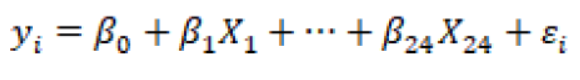
Where;

Y is the dependent variable; X1, X2, …, X24 is the independent variables in Table 1 and β0 , β1…., β24 are the unknown parameters.

Table 2 shows that a total number of independent variables are 21 out of which 12 are statistically significant on the bases of P-value at 0.05. The VIF values of 11 variables are greater than 10. It indicates that there is serious multicollinearity in the independent variables. The results of Model I are presented in Table 4.

Table 3 portrays that the Model I is significant. The coefficient of determination R²=0.82 shows the degree of linear-correlation of variables. On the other hand, the Durbin-Watson test value shows some problem of autocorrelation in the independent variables. Therefore, Model 1 is not suitable for the determinants of rice production.

Table 1: Explanation of Independent Variables for Model I.

Independent Variables Explanation	Sign	Independent Variables Explanation	Sign
Crop area in kanals	X1	Average temperature June	X13
Seed type (0=Home and 1= certified)	X2	Average temperature July	X14
Seed quantity in kg	X3	Average temperature August	X15
DAP Fertilizer used in kg	X4	Average temperature September	X16
Urea Fertilizer used in kg	X5	Average temperature October	X17
Other fertilizers used in kg	X6	Average temperature November	X18
Number of watering1	X7	Average humidity June	X19
Number of plowing	X8	Average humidity July	X20
Number of leveling2	X9	Average humidity August	X21
Use of Spray on crop (0=No and 1=Yes)	X10	Average humidity September	X22
Disease attack (0=No and 1=Yes)	X11	Average humidity October	X23
Average Rainfall	X12	Average humidity November	X24

 

Table 2: Summary of Model I monthly based on average temperature and humidity during crop period.

Model I					Collinearity Statistics
Variables	Unstandardized coefficients		t	Sig.	Tolerance	VIF
	Β	Std. Error
Constant	2.775	27.162	0.102	0.919
X1	0.144	0.058	2.484	0.013	0.86	1.163
X2	0.597	0.307	1.946	0.052	0.824	1.214
X3	0.464	0.105	4.417	0.000	0.651	1.535
X4	0.067	0.006	11.691	0.000	0.701	1.427
X5	0.053	0.005	10.069	0.000	0.694	1.442
X6	0.03	0.004	7.173	0.000	0.769	1.3
X7	0.289	0.053	5.445	0.000	0.467	2.143
X8	1.619	0.212	7.626	0.000	0.543	1.842
X9	0.736	0.281	2.619	0.009	0.571	1.753
X10	0.832	0.323	2.571	0.01	0.804	1.244
X11	-3.673	0.377	-9.747	0.000	0.558	1.794
X12	-0.104	0.381	-0.272	0.785	0.025	39.332
X13	-0.209	0.893	-0.234	0.815	0.016	61.162
X14	0.211	0.807	0.26	0.794	0.014	70.034
X15	1.034	1.045	0.989	0.323	0.028	35.956
X16	-0.074	0.099	-0.745	0.456	0.076	13.165
X17	0.075	0.092	0.811	0.417	0.145	6.888
X18	-0.194	0.094	-2.069	0.039	0.09	11.085
X19	-0.051	0.223	-0.229	0.819	0.011	91.083
X20	0.159	0.126	1.266	0.206	0.186	5.362
X21	-0.279	0.161	-1.733	0.084	0.035	28.971

Note: 1The meaning of no. of watering in the model is how much times the crop is irrigated minimum no. of irrigation is five times and maximum no. of irrigation is twenty-five; 2The meaning of no. of level is how much times the field is levelled after plowing for better irrigation and inputs used. The minimum no. of level is one and maximum no. of level is three.

Model II is based on average temperature and humidity during crop period and is defined as:

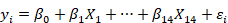
Where;

Y is the rice production in the mound (40 kg) per acre and is the independent variable. Descriptive statistics of all variables are given in Table 4.

Firstly, whether there are, or not outliers and influential observations in the data are examined by the plot of predicted values versus standardized residuals and Cook’s distance. The scatter plot of predicted values for Model II is presented in Figure 3. Figure 3 shows that all standardized residuals are between -3 and +3. It means that there are no outliers in the data. In addition, Figure 3 shows that the behavior of the dependent variable is constant and the rice yield is equally dissipated all over the sample data. It means that there is no heteroscedasticity. Then, the observations of which Cook’s values are greater than 4/n=4/516=0.008 are removed from the data.

Table 5 portrays the summary of stepwise multiple linear regression (MLR) and general fit statistics. The stepwise regression model is used to select automatically significant variables. It is found that the adjusted R² of our model is 0.849 with the R² = 0.853 which entails that the linear regression elucidates 85% of the variance in the data. The Durbin-Watson d = 1.997, which is between the two vital values of 1.5 < d < 2.5. Thus, we can ascertain that there is no first order linear auto-correlation in our MLR data.

Table 3: Summary of Model I based on monthly average temperature and humidity during crop period.

						Explained variation		Durbin- Watson
Model	Sum of squares	d.f	Mean square	F	Sig.	R square	Adjusted R Square
Regression	24814.532	21	1181.644	118.2	0.000	0.82	0.827	1.756
Residual	4940.200	494	10.000	-	-	-	-	-
Total	29754.732	515	-	-	-	-	-	-

 

Table 4: Independent Variables for Model II.

Independent Variables (Explanation)	Sign	Min.	Max.	Mean	St. deviation
Crop area in kanals	X1	0.25	9.70	4.8211	2.60112
Seed type (0=Home and 1= certified)	X2	-	-	-	-
Seed quantity in kg	X3	5	12	8.34	1.645
DAP Fertilizer used in kg	X4	0	100	34.93	28.844
Urea Fertilizer used in kg	X5	0	150	84.45	31.915
Other fertilizers used in kg	X6	0	125	20.74	38.462
Number of watering	X7	5	25	14.82	3.848
Number of ploughing	X8	2	8	4.34	0.891
Number of leveling	X9	0	3	1.54	0.657
Spray used on crop (0=No and 1=Yes)	X10	-	-	-	-
Disease attack (0=No and 1=Yes)	X11	-	-	-	-
Average rain fall	X12	2.92	12.86	9.7548	2.24323
Average temperature	X13	29	31	30.15	0.846
Average humidity	X14	49	58	52.37	2.803
Yield Acre in mounds	Y	5.21	48.21	24.3135	7.60106

 

Table 5: Stepwise multiple linear regression (MLR) results for Model II.

Model	R	R- Square	Adjusted R Square	Std. Error of the Estimate	Durbin- Watson
1	0.682	0.465	0.464	5.32176	-
2	0.797	0.636	0.634	4.39448	-
3	0.841	0.708	0.706	3.94063	-
4	0.884	0.781	0.779	3.41666	-
5	0.900	0.810	0.808	3.18394	-
6	0.907	0.823	0.821	3.07511	-
7	0.912	0.832	0.830	2.99775	-
8	0.915	0.838	0.835	2.95105	-
9	0.918	0.842	0.839	2.91427	-
10	0.920	0.846	0.843	2.88044	-
11	0.921	0.849	0.846	2.85607	-
12	0.923	0.851	0.847	2.84000	-
13	0.924	0.853	0.849	2.82471	1.997

 

Table 6 portrays the F-test, the linear regression F-test has the null hypothesis and found no linear relationship between the variables (in other words R² close to 0). The F-test is highly significant. Thus, it can be undertaken that a linear relationship is found between the variables in our model.

Table 6: Summary of Model II based on average temperature and humidity during crop period.

ANOVA
Model	Sum of squares	d.f	Mean square	F	Sig.
Regression	22082.758	13	1698.674	212.894	0.0000
Residual	3805.973	477	7.979	-	-
Total	25888.731	490	-	-	-

 

Table 7 portrays the estimates of MLR for Model II including the intercept and the levels of significance. As seen from Table 7, in our stepwise MLR analysis, a non-significant intercept but highly significant independent variables are found. Table 7 also shows that 13 independent variables are statistically significant on the bases of P-value at 0.05. It means that standard errors of all variables are less than 1 and also shows the stability in the dependent variable.

Table 7 also looks for multicollinearity in our MLR model. Therefore, tolerance should be higher than 0.1 (or VIF greater than 10) for all variables, which they are. There is no multicollinearity in the data since all VIF values smaller than 10. The three most important factors that affect the rice yield per acre in mounds are X4 (DAP Fertilizer used in kg), X11 (Disease attack) and X5 (Urea Fertilizer used in kg) respectively, where disease attack and average humidity have negatively affected and decreases the yield per acre in mounds.

Table 7: Summary of Model II based on average temperatures and humidity during crop period.

Model II					Collinearity statistics
Variables	Unstandardized Coefficients		t	Sig.
	B	Std. Error			Tolerance	VIF
Constant	3.631	4.883	0.744	0.457
X11	-3.668	0.333	-11.032	0.000	0.598	1.673
X8	1.686	0.194	8.688	0.000	0.594	1.684
X5	0.050	0.005	10.399	0.000	0.704	1.420
X4	0.068	0.005	12.906	0.000	0.735	1.361
X6	0.033	0.004	8.864	0.000	0.794	1.260
X3	0.381	0.092	4.120	0.000	0.725	1.380
X7	0.242	0.045	5.388	0.000	0.564	1.774
X1	0.164	0.052	3.162	0.002	0.877	1.140
X14	-0.295	0.062	-4.734	0.000	0.529	1.891
X9	0.932	0.249	3.746	0.000	0.631	1.586
X10	0.712	0.284	2.509	0.012	0.875	1.143
X13	0.439	0.169	2.594	0.010	0.787	1.271
X2	0.679	0.273	2.488	0.013	0.873	1.145

 

Figure 4 shows the predictive ability of the Model II. As seen from Figure 4, the predicted values obtained by Model II with the green line are very close to observed values with a blue line. It means that the data are nearly fitted by Model II.

Conclusions and Recommendations

The economy of Pakistan is highly agrarian based. The rank of Pakistan among biggest rice producers of the world is ten; whereas it stands at number four in world’s biggest exporters of rice. The empirical data of multiple linear regression (MLR) of the current study show that the behavior of all the variables is according to agriculture specification and ground realities. Two types of regression models are performed based on monthly average temperature and humidity during crop period and on average temperature and humidity during the crop period respectively. Projection behavior of the whole data is also examined. The reasonable results of projection level of estimates indicate that the Model 1 is not suitable for the determinants of rice production as there is no first-order linear auto-correlation in MLR data. Whereas Model II is acceptable for practical use as it shows that, 13 independent variables are statistically significant. It means that standard errors of all variables are less than 1 and also shows the stability in the dependent variable (Rice yield). Moreover, multicollinearity is not found in the data since all VIF values smaller than 10. The significance of the models and the variables are verified on the bases of the P-value at 0.05. The most significant factors that affect the rice yield per acre were crop area, seed type, seed quantity, number of watering, plowing, leveling, use of DAP and urea fertilizers etc. Whereas disease attack, spray use on crop have negatively affected and decreases the yield per acre in mounds. This means that these factors have a high share in imparting to the output yield of rice. Moreover, it is found that the average rainfall, temperature, and humidity in different months were not important factors that affecting the rice yield output. It can be concluded that the important factors of rice such as demand for the commodity needs and availability of labor to be appreciated to improve the yield output of rice. Thus, it can be helpful to the government to lessen the expenditures on subsidies and minimize the import of rice from other countries to boost the production and survival for the local rice growers.

Author’s Contributions

All the authors contributed equally to the design and implementation of the research, to the analysis of the results and to the writing of the manuscript.

References

Abedullah, S., S. Kouser and K. Mushtaq. 2007. Analysis of technical efficiency of rice production in Punjab (Pakistan). Pak. Eco. Soc. Rev. 45(2): 231-244.

Alam, I. 2017. Pakistan all set to become major rice producer: Cultivation of hybrid rice in Punjab can increase production to double digit. Available at: https://nation.com.pk/13-Oct-2017/pakistan-all-set-to-become-major-rice-producer.

Awan, A.G. and A. Alam. 2015. Impact of agriculture productivity on economic growth: A case study of Pakistan. Indus. Eng. Lett. 5(7): 27-33.

Azam, A. and M. Shafique. 2017. Agriculture in Pakistan and its impact on economy. Rev. Int. J. Adv. Sci. Tech. 103: 47-60. https://doi.org/10.14257/ijast.2017.103.05

Bhatti, F. 2015. A model based study of rice production: A case study of district Lodhran. M. Phil thesis, Dep. Stat. Islamia Univ. Bahawalpur, Pakistan.

Brazdik, F. 2006. Non-parametric analysis of technical efficiency: Factors affecting efficiency of west java rice farms. CERGE-EI working paper series no. 286. https://doi.org/10.2139/ssrn.1148203

Cook, R.D. 1977. Detection of influential observation in linear regression. Technometrics. 19(1): 15-18. https://doi.org/10.1080/00401706.1977.10489493

Javed, M.I., S.A. Adil, M.S. Javed and S. Hassan. 2008. Efficiency analysis of rice-wheat system in Punjab, Pakistan. Pak. J. Agric. Sci. 45(3): 95-100.

Kaloo, M.J., R. Patida and T. Choure. 2014. Production and productivity of rice in Jammu and Kashmir: An economic analysis. Int. J. Res. 1(4): 464-473.

Memon, N.A. 2013. Rice: Important cash crop of Pakistan. Pak. Food J. 21-23. Available at: http://www.foodjournal.pk/Sept-Oct-2013/Sept-Oct-2013-PDF/Exclusive-article-Rice.pdf.

Michel, L. and D. Makowski. 2013. Use of dynamic linear model for predicting crop yield trends in foresight studies on food Security 2013. UMR 211 INRA Agro Paris Tech BP01 Thiverval-Grignon, France.

NAU. 2018. Multiple regression. Northern Arizona University (NAU). Available at: fromoak.ucc.nau.edu/rh232/.../Regression/Multiple%20Regression%20-%20Handout.doc.

Qayyum, A., Pervaiz, M.K. 2010. Impact of weighted rainfalls on the yield of wheat in the Punjab, Pakistan. Afr. J. Agric. Res. 5(22): 3017-3025.

Rahman, S. 2011. Resource use efficiency under self-selectivity: The case of Bangladeshi rice producers. Aust. J. Agric. Res. Eco. 55(2): 273-290. https://doi.org/10.1111/j.1467-8489.2011.00537.x

Rawlings, J.O., S.G. Pantula and D.A. Dickey. 2001. Applied regression analysis: A research tool. Springer Sci. Bus. Media.

Raza, S.A., Y. Ali and F. Mehboob. 2012. Role of agriculture in economic growth of Pakistan. Int. Res. J. Fin. Eco. 83: 180-186.

Raza, M.A., L.Y. Fenga, A. Manaf, A. Wasaya and M. Ansar. 2018. Sulphur application increases seed yield and oil content in sesame seeds under rainfed conditions. Field Crops Res. 51-58. https://doi.org/10.1016/j.fcr.2017.12.024

Shah, M.A.A., A. Yasmeen and H. Qasim. 2014. Statistical analysis of agriculture crop data by two stage systematic sampling. Am.-Eurasian J. Agric. Environ. Sci. 14(10): 1026-1029.

Shaikh, F.M, M.B. Jamali, K. Shaikh and A.R. Abdi. 2011. WTO reforms and rice market in Pakistan. Int. J. Asian Soc. Sci. 1(3): 45-51.

Siyal, A.A., J. Dempewolf and I. Becker-Reshef. 2015. Rice yield estimation using Landsat ETM Data. J. App. Remote Sens. 9: 1-16. https://doi.org/10.1117/1.JRS.9.095986

Singh, D.P., D. Kumar, M.S. Paikra and P.S. Kusro. 2014. Developing statistical models to study the growth rates of Paddy crops in different districts of Chhattisgarh. Am. Int. J. Res. For. App. Nat. Sci. 5(1): 102-104.

Tun, Y.Y. and H. Kang. 2015. An analysis on the factors affecting rice production efficiency in Myanmar, J. East Asian Eco. Integ. 19(2): 167-188. https://doi.org/10.11644/KIEP.JEAI.2015.19.2.295

Turkan, S. and G. Özel. 2014. Modeling destructive earthquake casualties based on a comparative study for Turkey. Nat. Hazar. 72(2): 1093-1110. https://doi.org/10.1007/s11069-014-1059-x

Van der Eng, P. 2004. Productivity and comparative advantage in rice agriculture in southeast Asia since 1870. Asian Eco. J. 18(4): 345-370. https://doi.org/10.1111/j.1467-8381.2004.00196.x

Villano, R. and E. Fleming. 2004. Analysis of technical efficiency in a rainfed lowland rice environment in central Luzon Philippines using a stochastic frontier production function with a heteroskedastic error structure. Working paper no. (2004-15), Series in Agric. Res. Eco., Univ. New England.

Wanjari, R.H., K.G. Mandal, P.K. Ghosh, T. Adhikari and N.H. Rao. 2006. Rice in India: Present status and strategies to boost its production through hybrids. J. Sust. Agric. 28(1): 19-39. https://doi.org/10.1300/J064v28n01_04

World atlas. 2018a. 10 Largest rice producing countries 2018a. Available at: https://www.worldatlas.com/articles/the-countries-producing-the-most-rice-in-the-world.html.

World atlas.2018b. Top rice exporting and importing countries 2018b. Available at: https://www.worldatlas.com/articles/top-rice-exporting-and-importing-countries.html.