Investigation on Some Ectoparasites of Mesopotamian Spiny Eels (Mastacembelus mastacembelus) with Certain Data Mining Algorithms Based on the Effect of Weight and Sex

Mustafa Koyun1* and Şenol Çelik2

1Department of Biology, Faculty of Arts and Sciences, Bingol University, Bingol 12000, Turkey

2Department of Animal Science, Faculty of Agriculture, University of Bingol 12000, Turkey.

ABSTRACT

This study investigated the effect of Mastacembelocleidus heteranchorus (monogenea), Unio pictorum (glochidial larvae) and D. spathaceum (digenetic trematode) on the weight and sex of the host fish (Mastacembelus mastacembelus) by using some data mining algorithms. During this study, the fish weight (g) and length (mm) of 122 fish were measured. In addition, the distribution of M. heteranchorus and U. pictorum in each lamella of the gills and the distribution of D. spathaceum in the right and left eye lenses were evaluated. Two different algorithms (MARS and CHAID) were examined to evaluate the total fish weight, fish size, sex, season, station and recorded ectoparasites variables in host fish. In the study, MARS algorithm was formed to evaluate the effects of M. heteranchorus, U. pictorum recorded in the gills, and D. spathaceum recorded in eyes selected as independent variables. To estimate the MARS algorithm, goodness of fit statistics were examined. In order to determine the most suitable for each individual MARS model, different second, third and fourth-degree interactions were tried. In order to determine the most suitable model, it was taken into consideration that the cross-validity coefficient (GCV), square of error squared mean (RMSE) and Akaike Information Criteria (AIC) statistics were the minimum, the determination coefficient (R2) and Adj R2 values were maximum. In order to estimate the parasitic distribution of the host fish according to the total weight, the two different MARS (Multivariate Adaptive Regression Splines) model R2 values respectively; 0.973 and 0.989; Adj. R2 values were 0.967 and 0.985, RMSE values were 20.823 and 13.598, and AIC values 329.777 and 284.570 were found.

Article Information

Received 21 February 2019

Revised 01 May 2019

Accepted 19 June 2019

Available online 28 January 2020

Authors’ Contribution

MK planned the research, performed field surveys and wrote the article. ŞÇ analysed the data.

Key words

Mastacembelus mastacembelus, Mastacembelocleidus heteranchorus, Unio pictorum, Diplostomum spathaceum, MARS model, CHAID algorithms

DOI: https://dx.doi.org/10.17582/journal.pjz/20190221110209

* Corresponding author: [email protected]

0030-9923/2020/0002-0733 $ 9.00/0

Copyright 2020 Zoological Society of Pakistan

INTRODUCTION

Mesopotamian spiny eel, Mastacembelus mastacembelus is an endemic freshwater fish species of Euphrates and Tigris Rivers-Turkey (Coad, 1996, 2006) and in generally represents the whole characteristics of the Mastacembelidae family (Pala et al., 2010). It prefers slow-flowing waters and observed that when the water has cooled towards the end of autumn, this fish species moves to tributaries of rivers where temperature is partly high. (Geldiay and Balık, 2009; Jalali et al., 2008; Şahinoz et al., 2006).

It is seen that studies on the species belonging to the Mastacembelus genus are mostly carried out in the interior waters of Asia Minor and Far East (Kritsky et al., 2004; Jalali et al., 2008; Pazooki and Masoumian, 2012). Because of living in Asia Minor and Far East, several studies about this fish appear to be in Iran, Iraq, Syria and Turkey. It was described in Iran; from Tigris and Kor rivers, Persis basins and Qweik River, to the Persian Gulf in Helleh River, Greater Zab river, Darbandikhan Lake, Tigris and Euphrates River the region in Iraq, in southern Iran (Jouladeh-Roudbar et al., 2015; Bashě and Abdullah, 2010; Abdullah and Abdullah, 2015; Pazira et al., 2005). According to the previous records of Turkey; M. mastacembelus recorded from Tigris and Euphrates, Orontes River and their tributaries (Geldiay and Balik, 2009).

The Mesopotamian spiny eel is economically important because it is preferred by the people of the region as food (Kaçar et al., 2018). There is some related research on this fish at different locations in Turkey, these studies are known about more relevant about Mesopotamian spiny eel morphology, growth, and ecological aspects. (Karadede et al., 1997; Kılıç, 2002; Şahinoz et al., 2006a; Eroğlu and Sen, 2007; Şahinöz et al., 2006b; Oymak et al., 2009). But there was no known previous report about the parasitic fauna of this host fish species. Besides of these mentioned studies, there is only one limited note work in the Atatürk Dam Lake related of this fish (Öktener and Alas, 2009).

The target of this study is to determine the estimate of Mesopotamian spiny eel’s total weight, sex and size according to M. heteranchorus, U. pictorumum and D. spathaceum parasites by with MARS and CHAID algorithms.

 

MATERIALS AND METHODS

Present study was conducted in two major rivers of East Anatolian Region of Turkey, including four sampling sites at the both River; Tigris River, Site 1: (38° 22’ 50.52’’ N, 40° 41’ 02.56’’ E) Gonca Creek, Lice/Diyarbakır, Site2:(37°50’ 02.94’’N, 40° 41’ 52.10’’E) Bismil, and Euphrates River: (38°51’35.57’’N, 38°56’01.87’’E) Fatmalı, Keban/Elazığ, Murat River Site 1: (38°49’20.42’’N, 40°40’ 16.94’’E) Dikköy, Genç/ Bingöl, Site 1: (38°44’30.81’’N, 40°31’ 06.62’’E) Genç Bridge/Bingöl (Fig. 1).

 

In this study, a total of 122 fish, 56 male, and 66 females were studied and the total body weight (g), height (mm) and sex were recorded for each fish. On gills of each host fish (right 1, right 2, right 3 and right 4, left 1, left 2, left 3 and left 4) monogenean parasite M. heteranchorus, glochidial larvae U. pictorum and digenetic trematod D. spathaceum that located in the eyeball were counted separately and recorded.

Fish samples

The studied fish Mesopotamian spiny eel were obtained by the aid of fishermen from rivers Euphrates and Tigris years of 2014-2016 from four stations. All specimens were caught by gillnet, bag net, and fish trap during the spring to winter, samples of alive fishes were transported to the Research Laboratory, (Department of Biology/Zoology at University of Bingöl, Turkey) for parasitological examinations. After dissection, the stereomicroscopic observation was made on gills and eyes for the presence of parasites.

Parasitological examination

Fishes were examined with supervision organized by Bingöl University Animal Ethics Committee. The fish samples were dissected carefully and skin, gills, fins, eyes, gastrointestinal tracts and internal organs were examined for metazoan parasite species. The isolated parasites were collected, counted, and processed according to Gussev (1968) and Fernando et al. (1972). Parasites were identified according to Bychovskaya-Pavlovskaya (1962), Bauer (1985) and Pugachev et al. (2010).

In the first phase of the study, according to Model 1 and Model 2, the effect of the total weight, sex, number of recorded M. heteranchorus, U. pictorum and D. spathaceum factors were investigated by CHAID, Exhaustive CHAID, CART, and MARS algorithms. From these data, gender was categorical variable and other variables were held on considered as numerical variables.

Statistical calculations

One of the methods used to investigate the effects of independent variables on the dependent variable in the analysis of data is the MARS algorithm developed by Friedman (1991). The MARS method does not require any prior assumption about the underlying functional relationship between dependent and independent variables. Instead of a dynamic relationship between cause and effect variables are developed. The MARS technique not only examines the relationships of each independent variable with the dependent variable but also determines the interactions between the independent variables and the effect of interactions on the dependent variable (Hastie et al., 2001). The basis for MARS is the spline, a new mathematical process in complex curve drawings and function estimates. Chain smoothing is a method of controlling the non-parametric error variance obtained when two or more grade polynomials are used (Kaki et al., 2004). In MARS terminology, joining points of polynomials are called nodes (Hastie et al., 2008). Model setup takes place in two stages. In the first stage, MARS starts the model with only the fixed term and continuously adds the basic functions in pairs. Insertion continues until the number of basic functions reaches the highest level. In the creation of basic functions, the basic function of the same variable, which will be defined in the future, shows that the displacement between the dependent variable and the independent variable changes the inclination at the node point and the slope up to the zero nodes.

In the second stage, MARS uses a reverse step algorithm. The basic functions, which have the least contribution to the model at every stage, are discarded until the best sub-model is found. Determining the important independent variables and their interactions, the most suitable model with the least sum of error squares is created. The pruning algorithm is introduced by Craven and Wahba (1979) and is done by Friedman (1991) for Generalized Cross Verification (GCV), which is extended to MARS. GCV takes into account both the error of the debris and the model complexity and GCV;

C=1+cd

Calculated from equality. In the equation, n: The number of observations in the data set, d: Effective degree of freedom and the number of independent basic functions, A: The cost-complexity measure of the basic functions added and B: shows the number of regression models established by MARS model.

As a result of the calculations, it was found that the value of 2 <d <3 was the best for the C value. (Briand et al., 2004).

MARS Model consists of model parameters which are estimated by the least squares method with basic functions. General MARS’s model is as follows.

Here; k is number of nodes, K is number of basic functions, X is independent variable, βk is k. Coefficient of basic function, β0 is constant term in the model and αk is t. For the argument k. the basic function (Hill and Lewicki, 2006).

This function consists of the weighted sum of the cut-off parameter and one or more basic functions (Oguz, 2014).

To determine the basic functions, the MARS method uses a fragmented polynomial function. Regression cross-sections can be generated which can pass through the closest points to all values. The regression cross-sectional functions are a continuous function obtained by combining segmented polynomial basic functions in nodes. The constants in the basic functions are found by the least squares method. Basic functions.

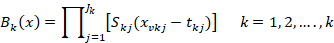
Defined as.

Here Jk: Interaction degree, [.]+ =max[0, .]+, Skj:E [±1], tkj: Node value, xvkj: Shows the value argument (Hill and Lewicki, 2006).

The MARS model is built by the basic functions of fitting different ranges of arguments. In MARS terminology, the joining points of the polynomials are called nodes and are indicated by a small letter “t”. MARS (x-t)+ and (t-x)+ shape used in the expansion of the elementary linear functions. Thus,

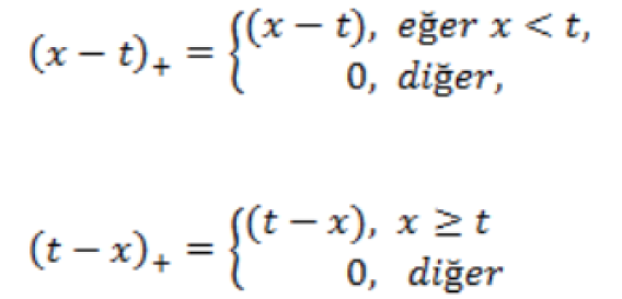
Equations are used (Hastie et al., 2008).

The MARS model creates flexible models using segmented linear regression and uses separate regression trends at different intervals of the argument to eliminate non-linear states. The points where the regression slope changes and passes from one interval to another is called a node (Chen and Lee, 2005).

CHAID analysis non-binary tress by splitting independent variables into categories based on chi-square statistic (Ratner, 2003). CHAID classifies a population into subgroups in a way that the variation in a dependent variable within groups is minimized and among groups is maximized (Dogan, 2003).

To determine the predictive performance of MARS and CHAID algorithms, the following goodness of fit criteria were investigated (Willmott and Matsuura, 2005; Takma et al., 2012; Ali et al., 2015):

1. Coefficient of Determination

2. Adjusted Coefficient of Determination

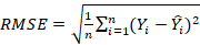
3. Root-mean-square error (RMSE) presented by the following formula:

4. Standard deviation ratio (SDratio):

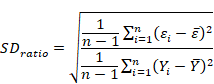
SD ratio estimates should be less than 0.40 for a good fit explained by some authors (Grzesiak et al., 2003; Grzesiak and Zaborski, 2012).

5. Akaike Information Criteria (AIC):

where: n is the number of cases in a set, k is the number of model parameters, Yi is the observed value of an output variable, Yip is the predicted value of an output variable, sm is the standard deviation of model errors, sd is the standard deviation of a response variable.

Statistical evaluations on MARS algorithm was specified using STATISTICA program (12.5 version).

 

RESULTS

Model 1

In order to estimate the live total weight in fish, MARS algorithm was formed by selecting fish size (mm), sex, total M. heteranchorus, U. pictorum numbers in gills and D. spathaceum numbers in eyepieces.

For estimating to the MARS algorithm, model compliance statistics were examined (Table I).

 

Table I. Model 1 goodness of fit criteria and GCV values according to order of interactions.

Order of int.	No. of BF	GCV	R2	Adj. R2	SD ratio	RMSE	AIC
2	11	1117.094	0.953	0.948	0.217	27.784	360.286
2	12	1012.282	0.955	0.950	0.213	27.365	358.675
3	23	1137.25	0.972	0.966	0.167	21.372	332.482
3	24	855.415	0.973	0.967	0.162	20.823	329.722
4	19	1058.054	0.969	0.963	0.177	22.756	339.131
4	19	865.116	0.969	0.963	0.177	22.756	339.131

BF: Basis functions, int: interactions.

 

According to the results of the goodness of fit shown in Table II, the best model was found to be the model with the 3rd degree 24 basic functions.

For this model; GCV = 855.415, R2 = 0.973, Adj. R2 = 0.967, SDratio = 0.162, RMSE = 20.823 and AIC = 329.722. The basic functions and their coefficients are given in Table II.

As seen in Table II, 24 basic functions, including fixed term, and a MARS model with three interactions (Model 1) were obtained.

The results obtained in this model are summarized as follows:

If the length is> 484 mm, the effect on the model is positive and the basic function coefficient is 2.275, If the length is≤484 mm, the effect on the model is negative and the basic function coefficient is -0.565, Length> 484 mm and M. heteranchorus> 0 if the model has a -0.068 effect, length> 484 mm and female fish have an effect on the model -3,232, If the effect is> 409 mm, the effect is 0.725, length> 409 mm, D. spathaceum> 8 and the effect of male fish on the model 0.077, and other basic functions and coefficients can be interpreted similarly.

Table II shows more clearly information that contains the basic functions and coefficients of the MARS model.

The main positive effect of the model is “max (0; Length-484)”. The coefficient for this basic function is 2.275. This was done by the basic function “max (0; 23-U. pictorum)*max (0; D. spathaceum-7)*max (0; Female-0)” (1.439) and the basic function “max (0; Length-553)*max (0; D. spathaceum-0)*max (0; Female-0)” (0.926), respectively. In other words, the basic function of “max (0; 23- U. pictorum)*max (0; D. spathaceum-7)*max (0; Female)” U. pictorum ≤ 23, D. spathaceum> 7 the contribution of female fish to the model is 1.439, Length> 553 and D. spathaceum> 0, which is the basic function of “max (0; Length-553)*max (0; D. spathaceum -0)*max (0; Female)”, is 0.926. The MARS equation for Model 1 is as follows. The main positive effect of the model was “max” (0; Length-484). Weight=161.287+2.275*max (0; Length-484)-0.565*max (0; 484-Length)-0.068*max (0; Length-484)*max (0; M. heteranchorus-0)-3.232*max (0;Length-484)*max (0; Female)+0.725*max (0; Length-409)+0.077*max (0; Length-409)*max (0; D. spathaceum-8)*max (0; Male)-5.714*max (0; Length-553)-0.019*max (0; Length-484)*max (0; M. heteranchorus-0)*max (0; D. spathaceum-8)+0.003*max (0;Length-484)*max (0; M. heteranchorus-0)*max (0;8-D. spathaceum)+0.033* max (0; Length-484)*max (0; 52-U. pictorum)+0.182*max (0;Length-553)*max (0; D. spathaceum -0)-4.242*max (0; Length-553)*max (0; M. heteranchorus-9)+0.166*max (0; Length-409)*max (0; U. pictorum-3)+0.926*max (0; Length-553)*max (0; D. spathaceum-0)*max (0; Female)- 0.163*max (0; Length-409)*max (0;U.pictorum-0)*max (0;Male)-0.162*max (0;Length-409)*max (0; U.pictorum-3)*max (0; Female)+0.005*max (0; Length-409)*max (0; U. pictorum-3)*max (0; D. spathaceum-8)+0.063*max (0; Length-522)*max (0; 0.023-U. pictorum)-1.149*max (0; U. pictorum-2.3)*max (0; D. spathaceum-8)*max (0; Male)+0.517*max (0; M. heteranchorus-0)*max (0; D. spathaceum-0)*max (0; Male)-1.575*max (0; 23-U. pictorum)*max (0; D. spathaceum-7)+1.439*max (0; 23-U. pictorum)*max (0; D. spathaceum-7)*max (0; Female)+0.035*max (0; Length-484)*max (0; M. heteranchorus-0)*max (0; Female).

In this equation, the values of height, M. heteranchorus, U. pictorum, D. spathaceum and live weight values which are expected to be different for the sex are given in Table III.

 

Table II. Model 1. Results of MARS algorithm for predicting live weight.

	Basic function	Coefficient
	Constant	161.287
BF1	max (0; Length-484)	2.275
BF2	max (0; 484-Length)	-0.565
BF3	max (0; Length-484)*max (0; M. heteranchorus- 0)	-0.068
BF4	max (0; Length-484)*max (0; Female-0)	-3.232
BF5	max (0; Length-409)	0.725
BF6	max (0; Length-409)*max (0; D. spathaceum-8)*max (0; Male)	0.077
BF7	max (0; Length-553)	-5.714
BF8	max (0; Length-484)*max (0; M. heteranchorus-0)*max (0; D. spathaceum-8)	-0.019
BF9	max (0; Length-484)*max (0; M. heteranchorus-0)*max (0; 8- D. spathaceum)	0.003
BF10	max (0; Length-484)*max (0; 52- U. pictorum)	0.033
BF11	max (0; Length-553)*max (0; D. spathaceum-0)	0.182
BF12	max (0; Length-553)*max (0; M. heteranchorus-9)	-4.242
BF13	max (0; Length-409)*max (0; U. pictorum-3)	0.166
BF14	max (0; Length-553)*max (0; D. spathaceum-0)*max (0; Female)	0.926
BF15	max (0; Length-409)*max (0; U. pictorum-0)*max (0; Male)	-0.163
BF16	max (0; Length-409)*max (0; U. pictorum-3)*max (0; Female)	-0.162
BF17	max (0; Length-409)*max (0; U. pictorum-3)*max (0; D. spathaceum-8)	0.005
BF18	max (0; Length-522)*max (0; 0.023-U. pictorum)	0.063
BF19	max (0; U. pictorum-2.3)*max (0; D. spathaceum-8)*max (0; Male)	-1.149
BF20	max (0; M. heteranchorus -0)*max (0; D. spathaceum-0)*max (0; Male)	0.517
BF21	max (0; 23-U. pictorum)*max (0; D. spathaceum-7)	-1.575
BF22	max (0; 23-U. pictorum)*max (0; D. spathaceum-7)*max (0; Female)	1.439
BF23	max (0; Length-484)*max (0; M. heteranchorus-0)*max (0; Female)	0.035

 

Table III. Estimated Weight values based on independent variable values.

Length	M. heteranchorus	U. pictorum	D. spathaceum	Sex	Weight
300	15	11	1	Male	65.054
325	6	9	0	Female	71.434
350	14	12	2	Male	100.025
400	20	15	5	Female	113.818
425	4	7	3	Male	138.089
450	50	40	10	Female	194.128
475	35	38	20	Male	541.059
500	0	0	0	Female	239.483
550	23	17	9	Male	415.150
600	5	8	3	Female	312.658
650	2	1	0	Male	563.224

 

As can be considered in Table III, for example, the length of the fish is 550 mm, M. heteranchorus parasite number 23, U. pictorum 17, D. spathaceum 9 and for calculating the live weight of a female fish, when the given values are replaced in this equation, the result is estimated 415.150 g. For Model 1, when parent node: Child node=6:3 is received, the goodness of fit for generating the CHAID algorithm R2=0.920, Adj. R2=0.918, SDratio=0.284, RMSE=36.490 and AIC=389.172 were found to be. The decision tree of the CHAID algorithm is given in Figure 2. When MARS and CHAID algorithms are compared in Model 1, it is seen that MARS algorithm is better when model performance is considered as a criterion.

Model 2

To estimate the live weight in fish, the numbers of M. heteranchorus and U. pictorum on the left and right lamellae of the gills, and D. spathaceum numbers recorded in the eyes were selected as independent variables and MARS and CHAID algorithms were created.

Model compliance statistics used to estimate the MARS algorithm are given in Table IV.

 

Table IV. Model 2 goodness of fit criteria and GCV values according to order of interactions (weight*).

Order of int.	Num. of BF	GCV	R2	Adj. R2	SDratio	RMSE	AIC
2	16	991.773	0.966	0.961	0.184	23.587	342.933
3	31	899.285	0.986	0.982	0.117	15.056	295.360
4	29	646.076	0.989	0.985	0.106	13.598	284.570

 

 

The results of the MARS model including the basic functions and coefficients are presented in Table V. The MARS model with 29 basic functions and 4 interactions are chosen as the most suitable model. GCV=646.076, R2=0.989, Adj. R2=0.985, SDratio=0.106, RMSE=13.598 and AIC=284.570 have been determined for this model.

M. heteranchorus_r: distribution in M. heteranchorus right gill lamella, M. heteranchorus_l: distribution in the

 

Table V. MARS algorithm estimated results.

	Basic function	Coefficient
	Constant	164.697
BF1	max (0; 484-Length)	-0.587
BF2	max (0; Length-484)*max (0; M. heteranchorus_l-0)	-0.192
BF3	max (0; Length-484)*max (0; 4-D. spathaceum_l)	-2.207
BF4	max (0; Length-484)*max (0; D. spathaceum_r-0)*max (0; D. spathaceum_l-4)	-0.007
BF5	max (0; Length-484)*max (0; U. pictorum_l-1)	0.418
BF6	max (0; Length-484)*max (0; 1- U. pictorum_l)	0.313
BF7	max (0; Length-484)*max (0; 1- U. pictorum_l)*max (0; female)	0.158
BF8	max (0; Length-409)	0.882
BF9	max (0; Length-484)*max (0; M. heteranchorus_l-0)*max (0; 4-D. spathaceum_l)	0.047
BF10	max (0; Length-484)*max (0; M. heteranchorus_l-0)*max (0; U. pictorum_r-0)*max (0; D. spathaceum_l-4)	0.069
BF11	max (0; Length-484)*max (0; U. pictorum_r-0)*max (0; 1- U. pictorum_l)	-0.053
BF12	max (0; Length-484)*max (0; U. pictorum_r-2)*max (0; 1- U. pictorum_l)*max (0; female)	0.089
BF13	max (0; Length-484)*max (0; 2- U. pictorum_r)*max (0; 1- U. pictorum_l)*max (0; female)	-0.262
BF14	max (0; Length-484)*max (0; 1- U. pictorum_l)*max (0; 4-D. spathaceum_l)	-0.663
BF15	max (0; Length-484)*max (0; U. pictorum_l-1)*max (0; male)	-0.347
BF16	max (0; Length-484)*max (0; 19- U. pictorum _r)*max (0; 4-D. spathaceum_l)	0.446
BF17	max (0; Length-484)*max (0; M. heteranchorus_r-0)*max (0; U. pictorum_r-19)*max (0; 4-D. spathaceum_l)	0.396
BF18	max (0; Length-484)*max (0; U. pictorum_r-0)*max (0; 1- U. pictorum_l)*max (0; D. spathaceum_r-0)	0.028
BF19	max (0; Length-484)*max (0; U. pictorum_r-0)*max (0; 1- U. pictorum_l)*max (0; D. spathaceum_l-0)	-0.018
BF20	max (0; Length-484)*max (0; M. heteranchorus_l-0)*max (0; U. pictorum_r-19)	0.381
BF21	max (0; Length-484)*max (0; 1- U. pictorum_l)*max (0; 4-D. spathaceum_l)*max (0; female)	0.093
BF22	max (0; Length-409)*max (0; D. spathaceum_r-0)	-0.047
BF23	max (0; Length-484)*max (0;M. heteranchorus_l-0)*max (0; D. spathaceum_r-0)*max (0; D. spathaceum_l-4)	-0.022
BF24	max (0; Length-409)*max (0; 19- U. pictorum_r)	-0.027
BF25	max (0; Length-409)*max (0;M. heteranchorus_r-2)*max (0; U. pictorum_r-19)	-0.081
BF26	max (0; Length-484)*max (0; M. heteranchorus_r-0)*max (0; U. pictorum_l-1)*max (0; 4-D. spathaceum_l)	0.008
BF27	max (0; Length-409)*max (0;M. heteranchorus_l-0)*max (0; D. spathaceum_r-0)*max (0; male)	0.023
BF28	max (0; Length-409)*max (0; 2-M. heteranchorus_r)*max (0; U. pictorum_r-19)*max (0; D. spathaceum_r-0)	-0.002

left gill lamella of M. heteranchorus, dispersion in U. pictorum_r: U. pictorum right gill lamella, distribution in U. pictorum_l: U. pictorum left gill lamella, D. spathaceum-r: D. spathaceum in the right eye, D. spathaceum-l: D. spathaceum in the left eye.

 

According to these results, the MARS equation of Model 2 is as follows.

Weight*=164.697-0.587*max (0; 484-Length)-0.192*max (0;Length-484)*max (0; M. heteranchorus l-0)-2.207*max (0; Length-484)*max (0; 4-D. spathaceum_l)-0.007*max (0; Length-484)*max (0; D. spathaceum_r-0)*max (0; D. spathaceum_l-4)+0.418*max (0; Length-484)*max (0; U. pictorum_l-1)+0.313*max (0; Length-484)*max (0; 1- U. pictorum_l)+0.158*max (0; Length-484)*max (0; 1-U. pictorum_l)*max (0; female)+0.882*max (0; Length-409)+0.047*max (0; Length-484)*max (0; M. heteranchorus_l-0)*max (0; 4-D. spathaceum_l)+0.069*max (0; Length-484)*max (0; M. heteranchorus_l-0)*max (0; U. pictorum_r-0)*max (0; D. spathaceum_l-4)-0.053*max (0; Length-484)*max (0; U. pictorum_r-0)*max (0; 1-U. pictorum_l)+0.089*max (0; Length-484)*max (0; U. pictorum_r-2)*max (0; 1- U. pictorum_l)*max (0; female)-0.262*max (0; Length-484)*max (0; 2- U. pictorum_r)*max (0; 1- U. pictorum_l)*max (0; female)-0.663*max (0; Length-484)*max (0; 1- U. pictorum_l)*max (0; 4-D. spathaceum_l) - 0.347*max (0; Length-484)*max (0; U. pictorum_l-1)*max (0; male-0)+0.446*max (0; Length-484)*max (0; 19- U. pictorum_r)*max (0; 4-D. spathaceum _l)+0.396*max (0; Length-484)*max (0; M. heteranchorus_r-0)*max (0; U. pictorum_r-19)*max (0; 4-D. spathaceum_l)+0.028*max (0; Length-484)*max (0; U. pictorum_r-0)*max (0; 1- U. pictorum_l)*max (0; D. spathaceum_r-0)-0.018*max (0; Length-484)*max (0; U. pictorum_r-0)*max (0; 1- U. pictorum_l)*max (0; D. spathaceum_l-0)+0.381*max (0; Length-484)*max (0; M. heteranchorus_l-0)*max (0; U. pictorum _r-19) + 0.093*max (0; Length-484)*max (0; 1- U. pictorum_l)*max (0; 4-D. spathaceum_l)*max (0; female)-0.047*max (0; Length-409)*max (0; D. spathaceum_r-0) - 0.022*max (0; Length-484)*max (0; M. heteranchorus_l-0)*max (0; D. spathaceum_r-0)*max (0; D. spathaceum_l-4) - 0.027*max (0; Length-409)*max (0; 19- U. pictorum_r) - 0.081*max (0; Length-409)*max (0; M. heteranchorus_r-2)*max (0; U. pictorum_r-19) + 0.008*max (0; Length-484)*max (0; M. heteranchorus_r-0)*max (0; U. pictorum_l-1)*max (0; 4-D. spathaceum_l)+0.023*max (0; Length-409)*max (0; M. heteranchorus_l-0)*max (0; D. spathaceum_r-0)*max (0; male) - 0.002*max (0; Length-409)*max (0; 2-M. heteranchorus _r)*max (0; U. pictorum_r-19)*max (0; D. spathaceum_r-0)

When the results are examined, for example, live weight, “max (0; 484-Length)” in the basic function Length 484 mm in the case of -0.587 times negative, “max (0; Length-484) *max (0; M. heteranchorus_l-0)” In the basic function Length> 484 mm and M. heteranchorus_l>0 was while the live weight of fish was affected by -0.192 times negative.

While the basic function is “max (0; Length-484) * max (0; U. pictorum_l-1)”, that is, in the case of Length>484 mm and U. pictorum-1>1, the effect on live weight is positive and this effect is 0.418.

The basic function is “max (0; Length-484) * max (0; 1- U. pictorum_l) * max (0; female-0)” and the contribution to model is 0.313. That means Length>484 mm, U. pictorum -l≤0 and the effect of female fish on the model is positive and this basic function coefficient is 0.313. Other basic functions and coefficients can be interpreted in a similar way according to the results given in Table V. Besides for Model 2, the values of height, M. heteranchorus, U. pictorum, D. spathaceum and live weight values which are expected to be different for the sex are displayed in Table VI.

For the Model 2, the parent node: Child node=6:3 is obtained from the goodness of fit for the generated CHAID algorithm, R2=0.919, Adj. R2=0.917, SDratio=0.284, RMSE=36.386 and AIC=386.433. The decision tree of the CHAID algorithm is presented in Figure 3.

 

Table VI. Estimated body weight values based on independent variable values.

Length	1	2	3	4	5	6	Sex	Weight
300	5	2	18	4	0	1	Male	56.749
350	15	5	7	8	2	0	Female	86.083
400	10	8	11	9	1	4	Male	115.417
450	8	15	9	12	5	3	Female	160.026
500	0	10	3	13	6	5	Male	286.234
550	16	11	4	1	0	6	Female	496.525
600	11	13	7	5	6	4	Male	618.470

1-M. heteranchorus-r, 2-M. heteranchorus-l, 3-U. pictorum-r, 4-U. pictorum-l, 5-D. spathaceum –r, 6-D. spathaceum-l.

 

DISCUSSION

In recent years, there are some limited studies on the MARS model in other animal husbandry areas except the fishery. Aytekin et al. (2018) used the MARS algorithm for predicting the live weight of young bulls in hybrid and exotic breeds. The authors stated that the MARS algorithm could provide a new perspective on the indirect selection criteria for breeding in animal husbandry. Aksoy et al. (2018), in the beekeeping study to estimate the honey production CART, CHAID and MARS algorithms were investigated comparatively. It is stated that the MARS algorithm performs better than other methods.

In some studies, it has been shown that using the MARS method, socioeconomic, biological determinants of beekeeping and different factors affect the honey yield per each hive. Therefore, it is recommended that the impact of socioeconomic and biological determinants on yield can be evaluated together for future studies. Erturk et al. (2018) studied the MARS model on factors affecting live weight in male and female cattle.

In the study of the authors, it was expressed that the average live weight per plant could change with the interaction of the influential factors entering the MARS prediction equation in fattening cattle. Karadas et al. (2017) using some morphological characteristics of Mengali sheep, for live weight estimation CHAID and MARS algorithms, were investigated comparatively. Researchers have explained that the MARS algorithm is more informative and powerful in predicting the live weight of sheep.

Celik et al. (2018) In Turkish Greyhound dogs, they investigated the live weight estimation by comparing some CART and MARS algorithms by using some body characteristics and explained that MARS algorithm is a more suitable model and it gives better results in predicting the live weight of dogs.

Eyduran et al. (2017) for estimating Mengali Sheep’s body weight by taking advantage of some body measurements feature, the MARS model was worked. In their study researchers reported that the MARS model gave good results in terms of compliance criteria. In addition, they suggested that the MARS model might be a good choice to examine the relationship between body weight and testicular measurements in identifying more produced Mengali rams.

Şahin et al. (2018) With the MARS Algorithm, it has used the global irradiation parameters to estimate the location of migratory birds. According to the eligibility criteria, the MARS model has shown very good results. A similar study was expressed in places of migratory birds for future studies related to global warming could give an idea about the scope of the global irradiation parameters.

 

CONCLUSION

According to the total weight of the Mesopotamian spiny eels, the highest infection effect of all three parasitic species in the Model 1 was in Length>484 mm, while in Model 2, Length>409 mm. In shortly, total weight and changes in fish size were affected by parasite infection intensity. In the CHAID algorithm, it was observed that fish size affected by total weight and intense parasites. Consequently, it is understood that data mining methods are very good and appropriate to predict the dependent variable. In this study, the effects of parasites on total weight with the interactive MARS model are explained. In line with the criteria of goodness of fit, the MARS model was found to be a very good model in estimating the total weight in this study as in other animal husbandry studies.

 

ACKNOWLEDGEMENT

This study was supported by Bingöl University with a project of BAP-35-235-2015.

 

Statement of conflict of interest

The author declares there is no conflict of interest.

 

REFERENCES

Abdullah, Y.S. and Abdullah, S.M.A., 2015. Some observations on fishes and their parasites of Darbandikhan Lake, In North Iraq. Eur. Sci. J., Special edition: 409-417.

Aksoy, A., Erturk, Y.E., Erdoğan, S., Eyduran, E. and Tariq, M.M., 2018. Estimation of honey production in beekeeping enterprises from Eastern Part of Turkey through some data mining algorithms. Pakistan J. Zool., 50: 2199-2207. https://doi.org/10.17582/journal.pjz/2018.50.6.2199.2207

Ali, M., Eyduran, E., Tariq, M.M., Tirink, C., Abbas, F., Bajwa, M.A., Baloch, M.H., Nizamani, A.H., Waheed, A., Awan, M.A., Shah, S.H., Ahmad, Z. and Jan, S., 2015. Comparison of artificial neural network and decision tree algorithms used for predicting live weight at post weaning period from some biometrical characteristics in Harnai Sheep. Pakistan J. Zool., 47: 1579-1585.

Aytekin, İ., Eyduran, E., Karadas, K., Akşahan, R. and Keskin, İ., 2018. Prediction of fattening final live weight from some body measurements and fattening period in young bulls of crossbred and exotic breeds using MARS data mining algorithm. Pakistan J. Zool., 50: 189-195. https://doi.org/10.17582/journal.pjz/2018.50.1.189.195

Bashě, S.K. and Abdullah, S.M.A., 2010. Parasitic fauna of spiny eel Mastacembelus mastacembelus from Greater Zab River in Iraq. Iran. J. Vet. Res., 11: 18-27.

Bauer, O.N., 1985. Guide for identification of parasites of the fresh water fish fauna of the USSR. Vol 2. Zoological Institute, Academy of Sciences of the USSR, Leningrad.

Briand, L.C., Freimut, B. and Vollei, F., 2004. Using multiple adaptive regression splines to understand trends in inspection data and identify optimal inspection rates. J. Sys. Softw., 73: 2-3. http://publica.fraunhofer.de/documents/N-6488.html https://doi.org/10.1016/j.jss.2004.01.015

Bychowskaya-Pavlovskaya, I.E., 1962. Key to parasites of freshwater fish of the USSR. Izdatel’stvo Akademii Nauk SSR. Moskva-Leningrad, pp. 919.

Celik, S. and Yilmaz, O., 2018. Prediction of body weight of Turkish Tazi dogs using data mining techniques: classification and regression tree (CART) and multivariate adaptive regression splines (MARS). Pakistan J. Zool., 50: 575-583. https://doi.org/10.17582/journal.pjz/2018.50.2.575.583

Coad, B.W., 1996. Zoogeography of the fishes of the Tigris-Euphrates Basin. Zool. Mid. East, 13: 51–70.

Coad, B.W., 2006. Freshwater fishes of Iran. http://www.briancoad.com (20 November 2006).

Craven, P. and Wahba, G. 1979. Smoothing noisy data with spline functions: Estimating the correct degree of smoothing by the method of generalized cross-validation. Numer. Math., 31: 377-403. https://doi.org/10.1007/BF01404567

Deichman, J., Eshgi, A., Haughton, D., Sayek, S. and Teebagy, N., 2002. Application of multiple adaptive regression splines (MARS) in direct response modelling. J. Interact. Mark., 16: 15-27. https://doi.org/10.1002/dir.10040

Doğan, I., 2003. Investigation of the factors which are affecting the milk yield in Holstein by CHAID analysis. Ankara Unıv. Vet. Fak., 50: 65-70. http://www.tarim.gov.tr/

Eroğlu, M. and Sen, D., 2007. Reproduction biology of Mastacembelus simack (Walbaum, 1792) inhabiting Karakaya Dam Lake (Malatya, Turkey). IJNES, 1: 69-73.

Ertürk, Y.E., Aksoy, A. and Tariq, M.M., 2018. Effect of selected variables identified by mars on fattening final live weight of crossbred beef cattle in Eastern Turkey. Pakistan J. Zool., 50: 1403-1412. https://doi.org/10.17582/journal.pjz/2018.50.4.1403.1412

Eyduran, E., Akkus, O., Kara, M.K., Tirink, C. and Tariq, M.M., 2017. Use of multivariate adaptive regression splines (MARS) in predicting body weight from body measurements in Mengali Rams. International Conference on Agriculture, Forest, Food, Food Sciences and Technologies (ICAFOF 15-17 May Cappadocia).

Fernando, C.H., Furtado, J.I., Gussev, A.V., Hanek, G. and Kakonge, S.A., 1972. Methods for the study of freshwater fish parasites. Department of Biology, University of Waterloo, Waterloo, Ontario, Canada. pp. 76.

Friedman, J.H., 1991. Multivariate adaptive regression splines. Ann. Stat., 19: 1-67. https://doi.org/10.1214/aos/1176347963

Geldiay, R. and Balik, S., 2009. Turkish freshwater fishes. VI. Print, Ege University Press, Izmir, Turkey.

Grzesiak, W. and Zaborski, D., 2012. Examples of the use of data mining methods in animal breeding. Chapter 3. pp. 303-324. https://doi.org/10.5772/50893

Grzesiak, W., Lacroix, R., Wójcik, J. and Blaszczyk, P., 2003. A comparison of neural network and multiple regression predictions for 305-day lactation yield using partial lactation records. Canadian J. Anim. Sci., 83: 307-310. https://www.researchgate.net/publication/270159514 https://doi.org/10.4141/A02-002

Gussev, A.V., 1968. Ammonium picrate as a fixative and mounting medium for slides of fish parasites. Zool. Z., 47: 935-936.

Hastie, T., Tibshirani, R. and Friedman J., 2008. The elements of statistical learning data mining, inference and prediction. 2nd Edition, Springer series in stat. pp. 745.

Hastie, T., Tibshirani, R. and Friedman, J., 2001. The elements of statistic al learning; data mining, inference and prediction. Springer Verlag, New York.

Hejnowska M., Pudyszak K. and Luter R., 1999. Wpływ pochodzenia na mikrostrukturę mięśnia piersiowego powierzchownego (m. pectoralis superficialis) i niektóre cechy użytkowe przepiórek japońskich. Appl. Sci. Rep. 45: 83-90.

Hill, T. and Lewichi, P., 2006. Statistics methods and applications. A comprehensive reference for science, industry and data mining. Stat Soft, Inc., USA. https://doi.org/10.1016/S1365-6937(06)71211-4

Jalali, B., Barzegar, M. and Nezamabadi, H., 2008. Parasitic fauna of the spiny eel, Mastacembelus mastacembelus Banks and Solander (Teleostei: Mastacembelidae) in Iran. Iran J. Vet. Med., 9: 158-161.

Jaturasitha, S., Srikanchai, T., Kreuzer, M. and Wicke, M., 2008. Differences in carcass and meat characteristics between chicken indigenous to northern Thailand (black-boned and Thai native) and imported extensive breeds (Bresse and Rhode Island Red). Poult. Sci., 87: 160-169. https://doi.org/10.3382/ps.2006-00398

Jouladeh-Roudbar A., Vatandoust S., Eagderi S., Jafari-Kenari S. and Mousavi-Sabet H., 2015. Freshwater fishes of Iran; an updated checklist. AACL Bioflux., 8: 855-909.

Kaçar, S., Başhan, M. and Oymak, S.A., 2018. Effect of season on the fatty acid profile of total lipids, phospholipids and triacylglycerols in Mastacembelus mastacembelus (Atatürk Dam Lake, Turkey). Grasas Aceites, 69: 1-9. https://doi.org/10.3989/gya.1108172

Kaki, B., Yeşilova, A. and Şen, C., 2004. Use of semi-parametric regression method in animal husbandry, IV. National Animal Science Congress, Oral Proceedings Program. pp. 26-32.

Karadas, K., Erturk, Y.E., Eyduran, E., Gursoy, A.K. and Tariq, M.M., 2017. Predictive performances of chaid and mars data mining algorithms in the establishment of relationship between live body weight and several morphological measurements of indigenous Mengali Sheep and its economic importance. International Conference on Agriculture, Forest, Food, Food Sciences and Technologies (ICAFOF 15-17 May 2017 Cappadocia).

Karadede, H., Cengiz, E.İ. and Ünlü, E., 1997. Investigation of heavy metal accumulation in Mastacembelus simack (Walbaum, 1792) in Atatürk Dam Lake. IX. National Aquaculture Symposium, Isparta. pp. 399-407

Kılıç, H.M., 2002. Research about biological features of Mastacembelus simack which is living in Sultansuyu Lake, Beyler Lake and Karakaya Dam. MSc thesis, Osmangazi University, Eskişehir, pp. 30.

Kritsky, D.C., Panndey, K.C., Agrawal, N. and Abdullah, S.M.A., 2004. Monogenoids from the gills of spiny eels (Teleostei: Mastacembelidae) in India and Iraq, proposal of Mastacembelocleidus gen. n., and status of the Indian species of Actinocleidus, Urocleidus and Haplocleidus (Monogenoidea: Dactylogyridae). Folia Parasitol., 51: 291-298. https://doi.org/10.14411/fp.2004.036

Lee, T.S. and Chen, I.F., 2005. A two-stage hybrid credit scoring model using artificial neural networks and multivariate adaptive regression splines. Expert Syst. Appl., 28: 743-752. https://doi.org/10.1016/j.eswa.2004.12.031

Oğuz, A., 2014. Multivariable adaptive regression chains and an application. Erzincan University, Institute of Science and Technology, Master Thesis, Erzincan.

Öktener, A. and Alaş, A., 2009. A parasitological study of fish from the Atatürk Dam Lake, Turkey. Bull. Eur. Ass. Fish Pathol., 29: 193-197.

Oymak, S.A., Kırankaya, Ş.G. and Doğan, N., 2009. Growth and reproduction of Mesopotamian spiny eel (Mastacembelus mastacembelus Banks & Solender, 1794) in Ataturk Dam Lake (Şanlıurfa), Turkey. J. appl. Ichthyol., 25: 488-490. https://doi.org/10.1111/j.1439-0426.2009.01234.x

Pala, G., Tellioğlu, A., Eroğlu, M. and Şen, D., 2010. The digestive system content of Mastacembelus mastacembelus (Banks and Solander, 11794) inhabiting in Karakaya Dam Lake (Malatya Turkey). Turk. J. Fish. aquat. Sci., 10: 229-233.

Pazira, A., Abdoli, A., Kouhgardi, E. and Yousefifard, P., 2005. Age structure and growth of the Mesopotamian Spiny Eel, Mastacembelus mastacembelus (Banks and Solander in Russell, 1974) (Mastacembelidae), in southern Iran. Zool. Mıddle East, 35: 43-47. https://doi.org/10.1080/09397140.2005.10638102

https://www.researchgate.net/publication/271669715

Pazooki, J. and Masoumian, M., 2012. Synopsis of the parasites in Iranian freshwater fishes. Iran J. Fish Sci., 11: 570-589. http://jifro.ir/article-1-629-en.html

Pugachev, O.N., Gerasev, P.I., Gussev, A.V., Ergens, R. and Khotenowsky, I., 2010. Guide to monogenoidea of freshwater fish of palaeartic and Amur regions (eds. P. Galli, O.N. Pugachev and D. Kristsky). Cover by Ledizioni- Ledipublishing, pp. 567.

Ratner, B., 2003. Statistical modeling and analysis for database marketing: Effective techniques for mining big data. Chapman and Hall, Washington. DC. https://doi.org/10.1201/9780203496909

Şahin, G., Eyduran, E., Turkoglu, M. and Şahin F., 2018. Estimation of global irradiation parameters at location of migratory birds in Iğdir, Turkey by means of MARS algorithm. Pakistan J. Zool., 50: 2317-2324. https://doi.org/10.17582/journal.pjz/2018.50.6.2317.2324

Şahinöz, E., Doğu, Z. and Aral, F., 2006. Development of embryos in Mastacembelus mastacembelus (Bank and Solender, 1794) (Mesopotamian spiny eel) (Mastacembelidae). Aquacul. Res., 37: 1611-1616. https://doi.org/10.1111/j.1365-2109.2006.01601.x

Şahinöz, E., Aral, F. and Doğu Z., 2007. Changes in Mesopotamian spiny eel, Mastacembelus mastacembelus (Bank & Solender in Russell, 1794) (Mastacembelidae) milt quality during a spawning period. Theriogenology, 67: 848–854. https://doi.org/10.1016/j.theriogenology.2006.11.001

Takma, C., Atil. H. and Aksakal, V., 2012. Comparison of multiple linear regression and artificial neural network models goodness of fit to lactation milk yields. Kafkas Univ. Vet. Fak. Derg., 18: 941-944.

Willmott, C. and Matsuura, K., 2005. Advantages of the mean absolute error (MAE) over the root mean square error (RMSE) in assessing average model performance. Clim. Res., 30: 79–82. https://doi.org/10.3354/cr030079