Research Article

Exchange Rate Volatility and Cotton Producer’s Behaviour: Evidence from Pakistan

Saad ud Din Khan1, Syed Rashid Ali1 and Sanam Wagma Khattak2*

1Department of Economics, University of Karachi, Pakistan; 2Department of Economics, University of Peshawar, Khyber Pakhtunkhwa, Pakistan

Received | January 22, 2019; Accepted | September 26, 2019; Published | November 26, 2019

*Correspondence | Sanam Wagma Khattak, Department of Economics, University of Peshawar, Khyber Pakhtunkhwa, Pakistan; Email: sanamah@uop.edu.pk

Citation | Khan, S.D., S.R. Ali and S.W. Khattak. 2019. Exchange rate volatility and cotton producer’s behaviour: Evidence from Pakistan. Sarhad Journal of Agriculture, 35(4): 1259-1265.

DOI | http://dx.doi.org/10.17582/journal.sja/2019/35.4.1259.1265

Keywords | Exchange rate volatility, Cotton production, Moving average standard deviation, Time series analysis, Pakistan

Introduction

Cotton is the most widely cultivated crop in Pakistan and among the top five exports from Pakistan. It accounted for 45% of the total exports. It also employed more than 35% of the total labour force in Pakistan (FAO, 2012; GOP, 2012). The basic purpose of this study is to study the behaviour of cotton producers in the amending situation of the exchange rate, whether the Pakistani cotton producer is risk-averse, risk-neutral or risk lover?

There is a global competition in the cotton export market, and exchange rate volatility can impact the cotton export as well. Pakistan cotton producers are very much concern about the exchange rate volatility because 45% of cotton exported, and exchange rate volatility can create uncertainty in profits. There is an immense literature on the exchange rate volatility and its impact on international trade. Exchange rate associates the domestic market with the rest of the world, and it describes the exchange power of a country (Aliyu, 2010a). But the impact of exchange rate volatility on trade in still imprecise as many studies found either a positive or negative relationship between these two variables (Ozturk, 2006). There are some results that (Arize, 1998; Chowdhury, 1993) support the hypothesis, while many results (Asseery and Peel, 1991; IMF, 1984) do not support.

The exchange rate is an important economic policy tool that can influence the production and exchange of tradable goods, especially cotton. It can influence tradable inputs and outputs such as fertiliser and raw cotton. The Pakistani government imposed import restrictions on cotton and jute in 1952 and in 1956, the rupee was devalued to promote exports, but exports decreased due to unfair incentives (Block, 1991).

For empirical analysis, initially, the stationarity checked through formal and informal methods. Then lag length criteria obtained through the lag length structure. Long run relationship is identified by using Johansen Co-integration Test. Vector Error Correction Model is used to obtain the long-run relationship at level and error coefficient is obtained through VECM, which shows adjustment pace of convergent toward equilibrium.

The results confirm a negative and significant relationship between exchange rate volatility and cotton production in Pakistan. It shows cotton producer’s risk-averse behaviour. The other determinants’ size and magnitude are in line with the hypothesis that is the ratio of capital per labour (kt) has a positive and significant effect on cotton production in Pakistan.

Volatility in the exchange rate has widely discussed in both theoretical as well as empirical literature since 1973. Studies like Either (1973) and Hooper and Kohlhagen, (1978) were the first who initiated the hypothetical foundation of exchange rate volatility and global trade relationship. But theoritcal literature found conflicting resutls between the Exchange Rate uncertainty and exports. For example, many studies found unfavourable relationship between international trade and exchange rate volatility (Either, 1973; Cushman, 1986; Peree et al., 1989) while Franke (1991) found positive relationship between Exchange rate volatility and international trade in developed countries.

Mustafa and Nishat (2004) analysed the Exchange rate volatility impact on export growth of Pakistan. The results confirm the negative and significant association between exchange rate volatility and exports growth in the long run as well as in the short run with the trading partners like the UK and US. Mustafa and Rashid (2018) found a negative effect of exchange rate volatility on different macroeconomic variables in Pakistan. Similarly, Paul et al. (2018) also finds negative relationship between exchange rate and different macroeconomic variables in Kuwait. Cho et al. (2002) examines the effect of Exchange Rate Volatility on wheat trade worldwide and finds mixed results. Samuel et al. (2014) studied the relationship between Exchange rate volatility and French beans exports from Kenya to trading partners. The results confirm the negative and significant relationship between Exchange Rate volatility and French beans exported to major trading partners. Similarly, Molina et al. (2013) also found a significant negative relationship between Exchange Rate Volatility and rice exports from Thailand to trading partners.

This study is peculiar in many ways. First, it investigates the effects of exchange rate risk on cotton production. Second, it gives sight of the nature of cotton producers and reflects their behaviour in the fluctuating exchange rate scenario. Third, this study takes yearly time-series data (1973-2018), which enhances the understanding of the relationship between exchange rate volatility and cotton production in Pakistan.

Materials and Methods

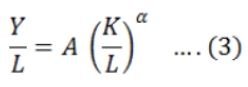
The objective of this study is to analyse the behaviour of cotton producers due to the exchange rate volatility in Pakistan by using the Cobb Douglas production function. In this study, cotton production is the dependent variable and exchange rate volatility as the independent variable. Additional variables like capital and labour as a factor of production also included. A similar generalised form of the model mentioned above also used by Sharma (2010) and Menyah and Wolde (2010). The Cobb Douglas production function is:

 

 

 

 

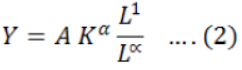
The generalised form of Cobb Douglas production function, including the exogenous variable, is as follows:

 

The line arise from the above model using the logarithmic transformation is:

Where;

‘A’ represents technology level and ln (A) = ao

 

The ‘t’ used in the subscript for time series and error term ‘u’ is used to add the model with the assumption of identically, independently and normally distributed.

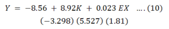
Here, yt represents the cotton production per capita, EXt represents the exchange rate volatility, kt represents capital per labour ratio, and ut is the error term. The expected sign of ‘a1’ is ambiguous (+/- ve) and ‘a₂’ is expected to be +ve.

Measurement of exchange rate volatility

Different methods found for the measurement of volatility, and they report different results in Economics literature (McKenzie, 1999). This study uses many studies used this method like (Kumar and Dhawan, 1991; Akther and Hilton, 1984; Gotur, 1985; Anjum and Nishat, 2006) moving average standard deviations method for the Exchange rate volatility and the formula is given in Equation 9,

 

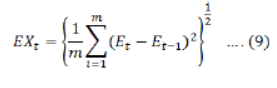
Here, bilateral nominal exchange at ‘t’ represented by ‘Et’, ‘m’ shows the order of moving average, bilateral nominal exchange rate at (t-1) represented by ‘Et-1’ period and EXt shows the volatility. The volatility in bilateral nominal exchange rate value at year-end of last four-year (m= 4) use a moving average method to compute the volatility.

Results and Discussion

This study uses annual time series data from 1973 to 2018. The data of cotton production collected from United States Department of Agriculture, Exchange rate data is collected from the International Financial Statistics (IFS-IMF), and the data of labour and capital formation have taken from the world development indicator (WDI). All the variables are in natural logarithm form, and the summary statistics presented in Table 1.

Initially, we check the stationarity of each variable through formal and informal methods, and the result is present in Table 2.

As variables, Yt, kt, and EXt are all stationary at the 1st difference, so we obtained residual through OLS and result is presented in equation no. 10. The residual obtained is stationary at level, i.e., I (0), the result presented in Table 2a, which shows that the Co-integration relationship exists among variables.

Table 1: Summary statistics.

	Y	K	EX
Mean	361.928	5.015952	2.977866
Standard Error	20.12818	0.026153	0.434468
Median	388.8153	5.039262	1.963125
Standard Deviation	136.5159	0.177379	2.946708
Sample Variance	18636.6	0.031463	8.683087
Kurtosis	-0.81252	0.349127	1.426862
Skewness	-0.48654	-0.72771	1.32685
Range	485.488	0.817085	12.42877
Minimum	106.6213	4.582915	0
Maximum	592.1093	5.4	12.42877
Sum	16648.69	230.7338	136.9818
No. of Observation	46	46	46

Source: Author’s calculation.

Table 2: Summary of the stationary level.

Variables	Augmented dickey-fuller test (ADF)				Phillip-perron test (PP)
	I (0)		I (1)		I (0)		I (1)
	C	C & T	C	C & T	C	C & T	C	C & T
Y	-1.860	-2.406	-9.178	-5.623	-1.624	-2.195	-9.877	-13.96
K	-1.185	-1.868	-5.907	-5.850	-1.287	-2.091	-6.078	-6.021
EX	-1.964	-2.513	-5.764	-5.847	-2.101	-2.639	-5.733	-5.830

Note: The critical values for ADF test with constant (c) and with constant and trend (C and T) 1%, 5% and 10% level of significance are -3.626, -2.945, -2.611and -4.394, -3.612, -3.243 respectively; The critical values for PP test with constant (c) and with constant and trend (C and T) 1%, 5% and 10% level of significance are -3.66, -2.93, -2.60 and -4.21, -3.52, -3.19 respectively; Source: Author’s calculation.

Table 2a: Summary of the stationary level of residual.

Variable	Augmented Dickey-Fuller Test (ADF)		Phillip-Perron Test (PP)
	I(0)		I (0)
	C	C and T	C	C and T
Error Term (ut)	-2.97	-3.69	-2.99	-3.65

Note: The critical values for ADF test with constant (c) and with constant and trend (C and T) 1%, 5% and 10% level of significance are -3.626, -2.945, -2.611and -4.394, -3.612, -3.243 respectively; The critical values for PP test with constant (c) and with constant and trend (C and T) 1%, 5% and 10% level of significance are -3.66, -2.93, -2.60 and -4.21, -3.52, -3.19 respectively; Source: Author’s calculation.

Table 3: Lag order selection criteria.

Lag	Log L	LR	FPE	AIC	SC	HQ
0	50.96691	NA	1.10e-05	-2.907086	-2.771039	-2.861310
1	84.66782	59.23189*	2.46e-06*	-4.404110*	-3.859925*	-4.221008*
2	89.95573	8.332473	3.13e-06	-4.179135	-3.226812	-3.858708
3	95.59540	7.861353	4.00e-06	-3.975479	-2.615017	-3.517725
4	107.7303	14.70894	3.57e-06	-4.165471	-2.396871	-3.570391

* indicates lag order selected by the criterion at 5% significant level; Source: Author’s calculation.

Lag length selection criteria shows the optimal lag length is 1, and the result presented in Table 3.

Then apply Johansen Co-integration Test and Johansen Co-integration trace statistics show 2 Co-integration equations while Eigen Max shows no co-integration equation. So according to trace statistics, Co-integration exists among variables. In other words, there exists a long-run relationship between variables. This result presented in Table 4.

Table 4: Johansen co-integration test.

Unrestricted Co-integration Rank Test (Trace)
Hypothesised		Trace	0.05
No. of CE(s)	Eigenvalue	Statistic	Critical Value	Prob.**
None *	0.459807	38.49080	29.79707	0.0039
At most 1 *	0.231867	15.70516	15.49471	0.0465
At most 2 *	0.148428	5.944815	3.841466	0.0148
Unrestricted cointegration rank test (Maximum eigenvalue)
Hypothesised		Max-Eigen	0.05
No. of CE(s)	Eigenvalue	Statistic	Critical Value	Prob.**
None *	0.459807	22.78564	21.13162	0.0290
At most 1	0.231867	9.760341	14.26460	0.2281
At most 2 *	0.148428	5.944815	3.841466	0.0148

Source: Author’s calculation.

To incorporate the long-run relationship among the variables, Vector Error Correction model used and result is shown below,

 

Now, the Vector Error Correction Model, (VECM) specification express the short-run relationship between variables yt, kt and EXt

 

Here βo is a constant term; β1 is the short-run coefficient of capital per unit labour β2 is the short-run coefficient of exchange rate volatility, and π is the coefficient of the estimated lagged residual and εt is the error term. The result obtained using the first lag of residual is:

Here we are concerned with a coefficient of lagged residual, i.e. -0.24128. It is the feedback effect or adjustment effect as the value is less than 0.5, which shows that the adjustment process is slow and negative sign shows that it is converging toward equilibrium. In other words, it tells how much disequilibrium is adjusted. The result of the variance decomposition is presented in Table 5. The result of variance decomposition shows that the system requires 10 years to converge toward equilibrium.

Table 5: Variance decomposition of yt.

Period	S.E.	it	kt	EXt
1	0.154869	100.0000	0.000000	0.000000
2	0.214262	89.16324	0.252783	10.58398
3	0.250783	84.89837	0.563598	14.53803
4	0.277307	80.42019	0.950092	18.62972
5	0.300175	79.01354	2.045853	18.94061
6	0.326648	76.80210	3.555520	19.64238
7	0.352644	75.44786	4.390437	20.16170
8	0.377127	74.04058	5.050038	20.90938
9	0.399387	73.16970	5.512532	21.31777
10	0.420530	72.45623	5.904135	21.63964

Source: Author’s calculation.

To check the stability in the regressive model, the CUSUM and CUSUMQ test is used. Cumulative sum (CUSUM) is used to check the stability of dependent variable through intercept term while Cumulative sum of Square (CUSUMQ) is used to check the stability of dependent variable through coefficients of parameters (sudden change in parameters). As our model consists one dependent variable ‘yt’ and two independent variables ‘kt’ and ‘EXt,’ the results obtained presented in Figures 1 and 2. The results of CUSUM shows that ‘yt’ is unstable, and have structural brake through intercept term while CUSUMQ shows the stability of ‘yt’ through coefficient parameters ‘kt’ and ‘EXt’.

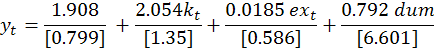
The cusum test shows instability in the estimated model, the structural break at point, 1985. The intercept dummy (dumt) variable is used to incorporate the pre and post effect to forecast the results. We use dum 0 (zero) for pre structural break and dum 1 for a post-structural break. The result estimated is as follows:

 

Pre 1985 model

 

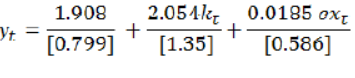
Post-1985 model

 

The results confirm that the intercept has changed from Pre, 1985 model to post, 1985 model.

Conclusions and Recommendations

Empirical estimates show that cotton production in Pakistan is negatively related to exchange rate volatility, and its significant effect means that an increase in volatility in the exchange rate has a tremendous impact on cotton production in Pakistan. The other variables, i.e., capital-labour ratio, are positive and significant, which is according to the theory. The result is contrary to the findings of (Aristotelous, 2001; Gagnon, 1993) but similar to (Haseeb and Ghulam, 2014). The negative effect shows that cotton producer is risk-averse.

It is concluded that Policymakers should have a concern at stabilising the exports market, which is likely to generate uncertain results. For the policy recommendations, attention should be given to exchange rate volatility as its impact is significant.

Novelty Statement

This study gives sight of the nature of cotton producers and reflects their behaviour in the fluctuating exchange rate scenario.

Author’s Contribution

Saad Uddin Khan conceived the idea, conducted the research, and analysed the data. Syed Rashid Ali collected the data, drafted and revised the manuscript. Dr. Sanam Wagma Khattak supervised and facilitated the research.

References

Arize, A.C. 1998. The effects of exchange-rate volatility on US export an empirical investigation. South. Econ. J. 62: 34-43. https://doi.org/10.2307/1061373

Akhter, M. and R.S. Hilton. 1984. Effects of exchange rate uncertainty of German and US Trade. Fed. Res. Bank N. Y. Q. Rev. 9: 7-16.

Aliyu, S.U. 2010. Exchange rate volatility and export trade in Nigeria: an empirical investigation. Appl. Finan. Econ. 20: 1071-1084. https://doi.org/10.1080/09603101003724380

Anjum, A. and N. Muhammad. 2006. The effect of exchange rate volatility on Pakistan’s exports. Pak. Econ. Soc. Rev. 44: 81-92. http://pu.edu.pk/home/journal/7/Volume_44_No_1_2006.html

Aristotelous, K. 2001. Exchange rate volatility, exchange rate regime, and trade volume: evidence from the UK–US Export Function (1989–1999). Econ. Lett. 72: 87–94. https://www.sciencedirect.com/science/article/pii/S0165176501004141

Asseery, A. and D.A. Peel. 1991. The effects of exchange rate volatility on exports: some new estimates. Economics Lett. 37: 73–177. https://www.sciencedirect.com/science/article/pii/0165176591901277

Block, S., 1991. The cotton economy of Pakistan. Agricultural policy analysis project, phase II, technical report No.121.

Cho, G., I. Sheldon and S. McCarriston. 2002. Exchange rate uncertainty and agricultural trade. Am. J. Agric. Econ. 84: 931-42. https://doi.org/10.1111/1467-8276.00044

Chou, W. 2000. Exchange rate variability and China’s exports. J. Comp. Econ. 28: 61-79. https://doi.org/10.1006/jcec.1999.1625

Chowdhury, A.R. 1993. Does the exchange rate volatility depress trade flows? Evidence from error correction models. Rev. Econ. Stat. 76: 700-06. https://doi.org/10.2307/2110025

Cushman, D.O. 1986. Has exchange risk depressed international trade? The impact of third-country exchange risk. J. Int. Money Finan. 5:361-379. https://www.sciencedirect.com/science/article/pii/0261560686900355.

Ethier, W. 1973. International trade and the forward exchange market. Am. Econ. Rev. 63(3): 494-503. Retrieved from http://www.jstor.org/stable/1914383.

FAO, 2012. Food and agriculture organization of the United Nations.

Franke, G. 1991. Exchange rate volatility and international trading strategy. J. Int. Money Finan. 10(2): 292–307. https://www.sciencedirect.com/science/article/pii/026156069190041H

Gagnon, J.E. 1993. Exchange rate variability and the level of international trade. J. Int. Econ. 34: 269–87. https://doi.org/10.1016/0022-1996(93)90050-8

GOP, 2012. Pakistan economic survey 2010e11. Economic advisory wing finance division. GoP, Islamabad, Pakistan. http://www.finance.gov.pk/

Gotur, P. 1985. Effects of exchange rate volatility on trade. IMF Staff Papers, 32: 475-512. https://doi.org/10.2307/3866807

Haseeb, M. and G. Rubaniy. 2014. Exchange rate instability and sectoral exports: Evidence from Pakistan. Paradigms. Res. J. Commerce, Econ. Soc. Sci. ISSN 1996-2800. 8: 31-49. https://doi.org/10.24312/paradigms080101

Hazlina. A.K., R. Masinaei and N. Rahmani. 2011. Long-term effects of bank consolidation program in a developing economy. J. Asia Pac. Bus. Innov. Tech. Manage. 1: 20-30. http://www.isbitm.net/journal/2/file/20160622123714_JAPBITM_v1_n1_3.pdf

Hooper, P. and S.W. Kohlhagen. 1978. The effect of exchange rate uncertainty on the prices and volume of international trade. J. Int. Econ. 8: 483-511. https://doi.org/10.1016/0022-1996(87)90001-8

IMF. 1984. Exchange rate volatility and world trade. IMF occasional paper, No. 28, Washington: Int. Monet. Fund. https://www.imf.org/en/Publications/Occasional-Papers/Issues/2016/12/30/Exchange-Rate-Volatility-and-World-Trade-195

Johansen, S. 1988. Statistical analysis of cointegration vectors. J. Econ. Dyn. Contr. 12: 231-254. https://doi.org/10.1016/0165-1889(88)90041-3

Khan, Z.M. 1990. Liberalisation and economic crisis in Pakistan. Financ. Tech. Int. Pak. https://aric.adb.org/pdf/aem/external/financial_market/Pakistan/pak_mac.pdf

Kumar, R. and R. Dhawan. 1991. Exchange rate volatility and Pakistani’s exports to the developed world, 1974-85. World Dev. 19:1225-40. https://doi.org/10.1016/0305-750X(91)90069-T

Menyah, K. and Y. Wolde-Rufael. 2010. Energy consumption, pollutant emissions and economic growth. S. Afr. Ener. Econ. 32: 1374-1382. https://doi.org/10.1016/j.eneco.2010.08.002

McKenzie and D. Michael. 1999. The impact of exchange rate volatility on international trade flows. J. Econ. Surv. 3: 71-106. https://doi.org/10.1111/1467-6419.00075

Molina, I.R., S. Mohanty, V. Pede and H. Valera. 2013. Modelling the effects of exchange rate volatility on thai rice exports. Selected paper, Ann. Meet. Agric. Appl. Econ. Assoc., Washington D.C. https://ageconsearch.umn.edu/record/150429?ln=en

Muhammad, H. and Ghulam, R. 2014. Exchange rate instability and sectoral export: evidence from Pakistan. Paradigms Res. J. Commerce Soc. Sci. Volume 8 issue 1. https://doi.org/10.24312/paradigms080101

Mustafa, K. and M. Nishat. 2004. The volatility of exchange rate and export growth in Pakistan: The structure and interdependence in regional markets. Pak. Dev. Rev. 43: 813-828. https://doi.org/10.30541/v43i4IIpp.813-828

Mustafa, K. and S.R. Ali. 2018. The macroeconomic determinants of remittances in Pakistan. Int. J. Bus. Manage. Finance Res. 1(1): 1-8. http://www.academiainsight.com/index.php/2641-5313/article/view/25

Ozturk, I. 2006. Exchange rate volatility and trade: A literature survey. Int. J. Appl. Econ. Quant. Stud. 3(1): 85- 102. https://papers.ssrn.com/sol3/papers.cfm?abstract_id=1127299. Pakistan economic survey (various issue)

Paul, F.H., S.R. Ali, R., Soomro, Q. Ali, S.K. Abbas. 2018. Exchange rate volatility and economic growth: Evidence from Kuwait. Eurasian J. Anal. Chem. 13(6): emEJAC181130. http://www.eurasianjournals.com/Exchange-Rate-Volatility-and-Economic-Growth-Evidence-from-Kuwait,104469,0,2.html

Peree, E. and A. Steinherr. 1989. Exchange rate uncertainty and foreign trade. Eur. Econ. Rev. 33: 1241-1264. https://www.sciencedirect.com/science/article/pii/0014292189900950. https://doi.org/10.1016/0014-2921(89)90095-0

Mwangi, S.C., L.E. Oliver, Mbatia and J.M. Nzuma. 2014. Effects of exchange rate volatility on french beans exports in Kenya. J. Agric. Econ., Ext. Rural Dev. Vol. 1(1) pp. 001-012, January 2014. http://www.repository.embuni.ac.ke/handle/123456789/355

Sharma, S.S., 2010. The relationship between energy and economic growth: Empirical evidence from 66 countries, Appl. Energy, Volume 87, Issue 11, pp. 3565-3574, (http://www.sciencedirect.com/science/article/pii/S0306261910002291) https://doi.org/10.1016/j.apenergy.2010.06.015

USDA. United States Department of Agriculture (USDA). Agric. Div. The USA. https://www.usda.gov/

WDI. World Development Indicators. Washington, D.C. The World Bank.