Curve Fitting with Nonlinear Regression and Grey Prediction Model of Broiler Growth in Chickens

Hande Kucukonder1, Pinar Celebi Demirarslan1*, Sezai Alkan2 and Özgür Baris Bırgul3

1Department of Business Administration, Bartın University, Ağdacı Campus, 74000, Bartın, Turkey.

2Department of Animal Science, Faculty of Agriculture, Ordu University, Ordu, Turkey

3Department of Animal Science, Faculty of Agriculture, Akdeniz University, Antalya, Turkey

ABSTRACT

In this study, it was aimed to model broiler growth curves of chickens with nonlinear regression analysis and grey prediction model. For this, the growth of 118 broilers was analyzed by using their weekly individual live weights from hatch to 49 day-old. In the analysis, nonlinear functions and Rolling-Grey Model (1,1) prediction method were used. The time-dependent growths of mixed sexes broilers were analyzed in the aspects of testing the parallelism of female and male growth samples, determining the best fitted growth model and designating the biological meaningful parameters (inflection point age, weight and growth rate) of growth functions. Analyses showed that the growth profiles of female and male chicks found not to be parallel using profile analysis, and the male chicks had a higher body weight than the females (P < 0.01) starting from 14-21st days until the end of experiment. For this reason, the prediction models were created separately and compared by MAPE (%) and accuracy rate (ρ) criteria in order to find out the most consistent growth model for female and male broiler chicks. The results indicate that Rolling-Grey Model (1,1) is more consistent than Von Bertalanffy, Gompertz and Logistic and can be used as an alternative to nonlinear regression models in growth analysis.

Article Information

Received 23 November 2018

Revised 01 March 2019

Accepted 19 April 2019

Available online 06 November 2019

Authors’ Contribution

HK designed and conducted the study. SA and OBB collected and recorded the data. HK and PCD analyzed the data and wrote the manuscript.

Key words

Nonlinear regression, Growth functions, Grey System Theory, Rolling-Grey Model (1,1), Broiler

DOI: https://dx.doi.org/10.17582/journal.pjz/2020.52.1.347.354

* Corresponding author: pdemirarslan@bartin.edu.tr

0030-9923/2020/0001-0347 $ 9.00/0

Copyright 2020 Zoological Society of Pakistan

INTRODUCTION

In terms of animal science, the growth is defined as the mass or volume change of a tissue or organism at a unit time. Improving the growth-related characteristics, particularly in meat production activities, is a priority goal. In animal breeding, growth is monitored and the effects of environmental factors on growth are followed up. The detected deviations in growth during the fattening period are not fancied and the negative effects are desirable to eliminate. Scientists have been studying on expressing growth over many years with different mathematical functions. To model the growth, nonlinear regression equations with the semi-empirical structure are usually used. These equations have 3 or 4 parameters and at least one parameter of the model has a biological meaning (France et al., 1996; Mendeş et al., 2007; Narinç et al., 2010a; Iqbal et al., 2019). The nonlinear regression models commonly applied in modeling of growth in poultry are 3-parameter Logistic, Von Bertalanffy, Gompertz models and 4-parameter Richards function. Moreover, Weibull, Von Bertalanffy, France, Morgan–Mercer–Flodin, Michaelis-Menten and Monomolecular are the other models that find few numbers for scientific studies. The studies carried out in poultry using growth models are divided into three categories as “election of the most compatible model”, “genetic structure of the growth curve” and “comparison of results of various applications with growth models”. While the analysis of growth with those models has been mostly carried out with the classical frequentist approach, probability-based methods (Bayesian) have also been used in recent years (Karaman et al., 2014, Fırat et al., 2016). Additionally, in order to model the growth, mixed effects model (Aggrey, 2009; Karaman et al., 2013), spline regression (Aggrey, 2002) and multi-stage models (Grossman and Koops, 1988) can also be used. A number of studies conducted on nonlinear functions that best define growth in broiler chicks (Narushin and Takma, 2003; Neme et al., 2006). In this study, it was aimed to investigate the growth of broiler chicks together with non-linear models with the Rolling-Grey Model (1,1) (RGM (1,1)) model based on grey system theory (GST). In the literature, although some studies using the method of grey relational analysis, which is a subset of the modelling based on the grey system theory, were found in animal science (Topal et al., 2016; Topal and Yağanoğlu, 2018), no finding about the use of RGM (1,1) method for modelling the growth in broiler chicks has been encountered during the research. In the first part of this study, the growth of 118 broiler chicks (mixed sexes) was analyzed with nonlinear functions (Von Bertalanffy, Gompertz and Logistic) using weekly individual weights from hatch to 7 week-old. In the second part, modeling of time dependent growth is given by using RGM (1,1) method based on GM (1,1) which is the basic model of grey prediction method. In the third part, the RGM (1,1), which is a special form of GP model, gives effective results was examined by comparing with nonlinear models. In comparison of model performances, the MAPE (%) and Accuracy rate (ρ) criteria were used.

MATERIALs AND METHODS

Animal material and husbandry

The study was carried out in the chicken coop in the Animal Husbandry Unit in Akdeniz University Department of Animal Science. In study, a total of 118 commercial broiler day old chicks were used. The chicks were grown in 4 deep-based base compartments. Additional heating is made to provide the optimum temperature in the experimental unit for the first 3 weeks. 23-hour lighting was implemented daily in the coop throughout the study. Starter feed (23% HP, 3200 ME kcal/kg) in the 0-3rd weeks and in the 4-7th weeks growing feed (20% HP, 3200 ME kcal/kg) are given as ad libitum to the birds (NRC, 1994). The body weights were measured with electronic scales with 0.01 sensitivity by attaching wing number to the one day-old chicks, and this process was repeated till the end of the experiment.

Profile analysis and nonlinear regression

The profile analysis technique was used primarily in determining the differences in male and female broilers according to body weight (weekly) values obtained at time points. This analysis is a particular usage of MANOVA (Srivastava, 1987).

In order to determine the most compatible growth function for broilers, Von Bertalanffy, Gompertz and Logistic nonlinear regression models were compared. The mathematical expressions of the growth models are given in Table 1. In the models, the parameters are as defined: β0 asymptotic (mature) symbolizes the weight, β1 refers the scaling (constant of integration), β2 stands for the sudden growth rate (per day) (Yang et al., 2006; Narinç et al., 2010b). The inflection point is the point that divides the curve into two parts in sigmoid models and that the best growth rate (Narinç et al., 2014). The inflection point age, weight for all three models and the equations representing the highest growth rate at these points are presented in Table I. The prediction of the model parameters was done by the Levenberg-Marquardt iteration method by SAS 9.1.3 NLIN procedure (SAS Ins., 2005).

Grey prediction model GM (1,1)

The main focus of grey system theory (GST) brought to literature by Deng in 1982 is its tendency towards establishing a mathematical relationship among the factors related to the data with reference to the behavioral data of the systems such as social, industrial, economical, ecological, agriculture, biological etc. This theory usually examines systems with few data and partially unknown variables (Liu and Lin, 2006). The basic philosophy of GST’s emergence is expressed in the way of predicting and solving an analysis of uncertain systems which cannot be resolved by fuzzy or stochastic methods with a limited number of data (Aydemir et al., 2013). One of the main areas of activity in GST is the grey prediction (GP) method.

In GST, the general notation of grey prediction models is given as GM (n,h). Here, n states the order of differential equation, while h refers to the number of variables so that GM (1,1) is a type of grey model with 1 variable in first order (Liu and Lin, 2006). GM (1,1) is a form of time series model with three basic operators, which are AGO (accumulated generating operation), IAGO (inverse accumulated generating operation) and grey modelling (Lee and Shih, 2011; Liu and Lin, 2010).

Table I.- The growth curve models and the coordinates of inflection point.

IPW, Inflection point weight; IPA, Inflection point age.

The prediction phase in this model consists of 6 steps presented as follows (Huang et al., 2015; Liu and Lin, 2006; Liu and Lin, 2010):

• Step 1: Establishing the initial sequences.

  r0 the original data set is shown as follows using the initial data set.

  

  • Step 2: Developing the AGO sequence (Conversion of the initial sequence to monotone increasing sequence)

  r0 sequence converted to the monotonically increasing r1 sequence and this sequence is formed by cumulative sums. r1 sequence is obtained as in Equation 3, which is an AGO.

  

  • Step 3: Establishing a first–order grey differential equation

  In this step, so as to find the GM (1,1) coefficients, the first-order grey differential equation is established as follows.

  

  When the equally weighted defuzzification method is used, it is found that α=0.5. However, equally weighted defuzzification method (α =0.5) is not always effective in uncertain systems. Therefore, the alpha value can vary to have the optimum value in order to increase the model performance and improve the prediction results (Li and Zhao, 2012).

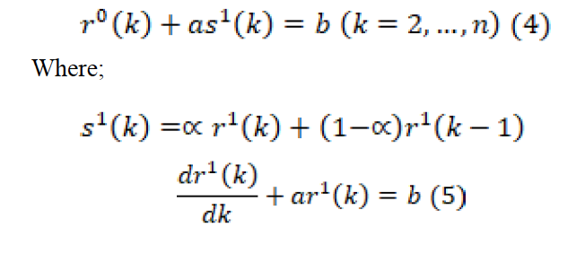
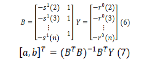
  • Step 4: Establishing the grey prediction equation (Calculation of model parameters)

  The least squares method (LSM) is exerted to predict the model parameters. In Equation 4, a parameter represents the evelopment coefficient, while b represents the drive coefficient or amount of greying. For parameter prediction, the s1(k)(k=2, …., n) values are used in the method of LSM given in Equation 7 by putting them in the form of B and Y matrices in Equation 6. The equations used to predict the values of a and b and the expansion of matrix forms in the equation are as shown below.

  

  • Step 5: Apply the IAGO to predicted values in order to obtain the solution at time k

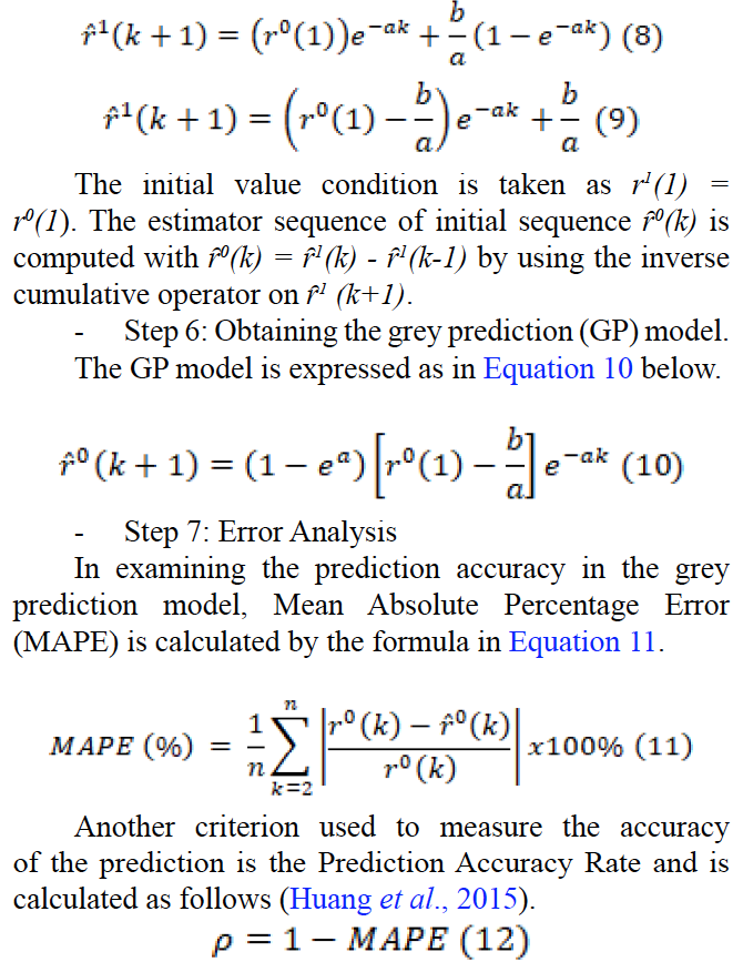
  The prediction equation at (k + 1) is obtained using the predicted values of the a and b parameters obtained by solving the first-order derivable equation shown in Equation 5.

  

  RGM (1,1)

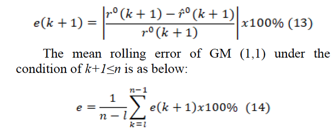
  RGM (1,1) is a Grey model that emerged to improve the conventional GM (1,1) model. It is necessary to

  have at least 4 past records in order to make predictions in the RGM (1,1). The main basis of RGM (1,1) is the establishment of a new model for each new consecutive forecast value. The model constantly updates itself by shifting the sequence for the predicted value. This shifting process is continued until k < n (Hsu, 2011). Examination of the prediction accuracy at each time point in the GP rolling model is calculated by the formula in Equation 13 (Hsu, 2011):

  

  Performance of the prediction models

  During the study, two criteria, namely MAPE (Equation 11) and the prediction accuracy (Equation 12), are used for examining the performance of the prediction models. According to Ma and Zang’s study, the prediction model gets high accuracy if MAPE gets close to zero, which suggests the model’s performance is good (Huang et al., 2015).

   

  RESULTS

  Nonlinear model results

  According to the MANOVA test statistic (Wilks’ Lambda = 0.0001) in the corresponding chart, sex profiles do not show parallelism. As a result of the analyzes carried out, it was determined that the difference in body weight between sexes first appeared between the 14-21st days (p<0.01) and continued to exist until the end of the trial.

  The growth samples of female and male broiler chicks were analyzed by Bertalanffy, Gompertz and Logistic functions and the growth curves of these models are displayed in Figure 1. The parameters of Bertalanffy, Gompertz and Logistic growth models, the correlations between parameters, the inflection point of age, and weight and growth rate values at this point are given in Table II.

  In terms of the β0 parameter representing the mature weight, higher values were estimated for male broiler chicks than for females in all three models. β0 values of Bertalanffy model are higher than other Gompertz and Logistic model values. In terms of β1 parameter representing the integration constant, the Logistic model showed more deviation values than other models. The predicted values for female and male broiler chicks in terms of the instantaneous growth rate parameter in Bertalanffy model are 0.028 and 0.024, respectively, while they are predicted in the Gompertz model as 0.048 and 0.045, respectively. The predicted values for the logistic model in terms of the parameter (0.106 and 0.104) were found to be quite higher than the other two models. The correlations of growth curve parameters were negative for β0-β1 and β0-β2, while they were found positive for β1-β2 in all models. In terms of inflection point ages, higher values were predicted for male broiler chickens than for females in each model. Similarly, in terms of inflection point weights and maximal increment rates, higher values were predicted for males than for females in all three models.

  The results of RGM (1,1)

  In the RGM (1,1) used to predict the time-dependent growth of female and male broiler chicks, different experiments were performed to determine the k and α coefficients. According to the result of these experiments, the number of data to be used in the growth prediction for

  
  

   

  Table II.- The parameter values of growth curve models, the correlations between parameters, the coordinates of inflection point.

  Sex	Model	β0	β1	β2	rβ0β1	rβ0β2	rβ1β2	IPA	IPW	Winc
  Female	Bertalanffy	5334	0.88	0.028	-0.79	-0.98	0.88	34.67	1580	66.37
  	Gompertz	3947	4.73	0.048	-0.70	-0.96	0.85	32.37	1456	69.90
  	Logistic	2924	31.62	0.106	-0.53	-0.85	0.87	32.58	1462	77.48
  Male	Bertalanffy	7677	0.89	0.024	-0.80	-0.99	0.87	40.91	2274	81.88
  	Gompertz	5172	4.95	0.045	-0.70	-0.96	0.84	35.54	1908	85.88
  	Logistic	3593	36.39	0.104	-0.54	-0.86	0.87	34.56	1796	93.42

   

  Table III.- RGM (1,1) prediction results.

  Obs	Time	Male				Female
  		Actual weight	RGM (1,1) Prediction	RGM (1,1) prediction coefficients	MAPE (%)	Actual weight	RGM (1,1) Prediction	RGM (1,1) prediction coefficients	MAPE (%)
  1	0	50.83				50,83
  2	7	134.14				133.84
  3	14	352.37				342.85
  4	21	766.99				711.56
  5	28	1276.12	k=5			1167.41	k=5
  6	35	1839.17	1853.7	a= -0.57; b = 109.3	0,79	1628.03	1624.41	a= -0.55; b = 106.3	0.22
  7	42	2446.9	2512.6	a= -0.44; b = 288.9	2,68	2127.53	2167.82	a= -0.41; b = 278.6	1.89
  8	49	2994.68	3143.58	a= -0.34; b = 572.7	4,97	2524.6	2676.174	a= -0.32; b = 537.7	6.00
  Mean MAPE (%)			2.81			Mean MAPE (%)		2.70
  Accuracy ρ (%)			97.19			Accuracy ρ (%)		97.3
  Predicting level			Excellent			Predicting level		Excellent
  α Coefficient			α = 0.621			α = 0.637

   

  Table IV.- The comparison of performances of prediction models.

  Sex	Model performance criteria	Von Bertalanffy MAPE (%)	Gompertz MAPE (%)	Logistic MAPE (%)	RGM (1,1) MAPE (%)
  Male	MAPE (%)	13.38	5.01	19.71	2.81
  	Accuracy ρ (%)	86.62	94.99	80.29	97.19
  	Predicting level	Qualified	Good	Unqualified	Excellent
  Female	MAPE (%)	13.59	4.88	16.51	2.71
  	Accuracy ρ (%)	86.41	95.12	83.49	97.29
  	Predicting level	Qualified	Excellent	Unqualified	Excellent

  Excellent: MAPE <0.01 and Accuracy >0.95; Qualified: MAPE < 0.10 and Accuracy >0.85; Good: MAPE <0.05 and Accuracy >0.09; Unqualified: MAPE ≥0.10 and Accuracy ≤0.85 (Huang et al., 2015)

  both female and male broiler chicks was determined as k= 5. The prediction results obtained by rolling GM (1,1) according to optimum k and α are presented in Table III.

  According to Table III, when the mean MAPE (%) and Accuracy rate (ρ) of the RGM (1,1) were examined together, these values were found to be higher than 95%. According to predicting level, it is observed that the RGM (1,1) gave quite successful results without estimating the actual values at different time points examined. The results of MAPE (%) and Accuracy rate (ρ, (%)) criteria used to compare model performances are given in Table IV. Accordingly, it was determined that the best prediction model is the Gompertz model, and it is followed by Von Bertalanffy and Logistic growth model in terms of MAPE (%) and Accuracy rate ρ (%) among the nonlinear functions included in the study. On the other hand, when both the MAPE (%) and Accuracy rate ρ (%) are evaluated together, it is seen that the lowest values belong to the RGM (1,1) for both female and male broiler chicks.

  DISCUSSION

  Many studies have shown that there is a difference between the body weights of female broilers and male broilers and those female broilers have less body weight values than males (Gous et al., 1999; Yakupoglu and Atil, 2001a; Aggrey, 2002; Santos et al., 2005; Narinç et al., 2007; Marcato et al., 2008). Narinç et al. (2007) reported that the Gompertz model β1 parameter values for slow growing female and male broiler chicks are 4.42 and 4.74, respectively, while for commercial broiler chicks 4.68 and 5.22, respectively. The values reported by Narinç et al. (2007) were found consistent with these research results. In this study, the predicted values of the β2 parameter of the Gompertz model were found higher than the predicted values for slow-growing broilers and then the findings of Wang and Zuidhoff (2004), while they were found compatible with the findings of Marcato et al. (2008). There are not many studies using Von Bertalanffy and Logistic models on the growth of broiler chicks.

  Yakupoğlu and Atil (2001a), who analyzed the growth in Cobb and Hubbard commercial broilers with Von Bertalanffy’s function, reported that β0, β1 and β0 parameters are 4923 g, 0.97 and 0.16, respectively for females, while for males 5156 g, 0.99 and 0.17, respectively. Darmani-Kuhi et al. (2003), who examine growth on a line developed for meat production with different models, reported that for Von Bertalanffy and Logistic models β0 parameter is 5159 g and 3739 g, respectively for females, while 5475 g and 4413 g respectively for males. In this study, the parameter predictions obtained by using Von Bertalanffy and Logistic model are close to the values reported by Yakupoğlu and Atil (2001a) and Darmani-Kuhi et al. (2003).

  In the growth analyzes carried out at with the data collected from the broilers at early ages (5-7 weeks), IPA values determined by the Gompertz model was found between 32.07-40.46 days by various researchers (Yakupoglu and Atil, 2001b; Marcato et al., 2008). Darmani-Kuhi et al. (2003) stated that IPA values are found 43, 43 and 46 days, respectively for male broilers, while 43, 42 and 45 days, respectively for female broilers by using Gompertz, Von Bertalanffy and Logistic functions. The IPA values determined in this study (female:32-35 days, male:35-41 days) were found consistent with the findings of researchers using growth data obtained from conventional system, while were found to be lower than the IPA values determined for broilers grown in an alternative system or for longer periods (Santos et al., 2005).

  The growth of male and female chicks was analyzed by RGM (1,1) as well as nonlinear functions. When the performances of Gompertz, Von Bertalanffy and Logistic functions compared with the RGM (1,1) according to MAPE (%) and Accuracy ρ criteria, it was seen that the RGM (1,1) produced more accurate and predicted results with higher accuracy. When the classification by Liu and Deng for the (-a) variant in the GM (1,1) is taken as basis (Huang et al., 2015), it can be said that the RGM (1,1) is appropriate for short-term predictions (for both female and male chicks) depending on the data structure used. The coefficient b, also referred to as the amount of greying in the same prediction model, reflects the changes that occurred or to be occurred in the data over the period studied, since it is based on the past knowledge of the data (Kayacan et al., 2010). Based on this information, it can be said that when the b coefficients of the prediction equations obtained for each time period for both female and male chicks are examined, the change in the growth rate of male chicks is more than that of females.

  Conclusion

  As a result, nonlinear functions and RGM (1,1) were analyzed for growth in broiler chicks in the present study. It is seen that RGM (1,1) created with previous 5 different points (k = 5) data from weekly measured growth data produced very similar results to actual values with lower error. It may therefore be advisable to use grey prediction models as an alternative to nonlinear models where limited data is obtained for purposes, such as monitoring the growth of the animals during the production process, taking precautions against adverse environmental effects, herd management, etc. On the contrary, if growth is being sought for breeding, the model to be used should be mechanistic and have biologically meaningful parameters. Thus, biological parameters such as model parameters, inflection point coordinates, absolute growth rate, and relative growth rate can be used in genotype breeding programs.

   

  Statement of Conflict of Interest

  Authors have declared no conflict of interest.

   

  REFERENCES

  Aggrey, S.E., 2002. Comparison of three nonlinear and spline regression models for describing chicken growth curves. Poult. Sci., 81:1782–1788. https://doi.org/10.1093/ps/81.12.1782

  Aggrey, S.E., 2009. Logistic nonlinear mixed effects model for estimating growth parameters. Poult. Sci., 88:276–280.

  Aydemir, E., Bedir, F.G. and Özdemir, G., 2013. Grey system theory and applications: a literature review. Suleyman Demirel Univ. J. Econ. Administ. Sci., 18:187-200.

  Darmani Kuhi, H., Kebreab, E., Lopez, S. and France, J., 2003. An evaluation of different growth functions for describing the profile of live weight with time (age) in meat and egg strains of chicken. Poult. Sci., 82:1536–1543. https://doi.org/10.1093/ps/82.10.1536

  Fırat, M.Z., Karaman, E., Basar, E.K. and Narinç, D., 2016. Bayesian analysis for the comparison of nonlinear regression model parameters: an application to the growth of Japanese quail. Brazilian J. Poult. Sci., 18:19-26. https://doi.org/10.1590/1806-9061-2015-0066

  France, J., Dijkstra, J., Thornley, J.H.M. and Dhanoa, M.S., 1996. A simple but flexible growth function. Growth Dev. Aging, 60:71–83.

  Gous, R.M., Moran, E.T., Stilborn, H.R., Bradford, G.D. and Emmans, G.C., 1999. Evaluation of the parameters needed to describe the overall growth, the chemical growth, and the growth of feathers and breast muscles of broilers. Poult. Sci., 78:12-21. https://doi.org/10.1093/ps/78.6.812

  Grossman, M. and Koops, W.J., 1988. Multiphasic analysis of growth curves in chickens. Poult. Sci., 67:33-42. https://doi.org/10.3382/ps.0670033

  Hsu, L.C., 2011. Using improved grey forecasting models to forecast the output of opto-electronics industry. Exp. Sys. Applic., 38:13879-13885. https://doi.org/10.1016/j.eswa.2011.04.192

  Huang, Y.F., Wang, C.N., Dang, H.S. and Lai, S.T., 2015. Predicting the trend of Taiwan’s electronic paper industry by an effective combined grey model. Sustainability, 7:10664-10683. https://doi.org/10.3390/su70810664

  Iqbal, F., Waheed, A., Huma, Z., Faraz, A., 2019. Nonlinear growth functions for body weight of Thalli sheep using bayesian inference. Pakistan J. Zool., 51: 1421-1428. http://dx.doi.org/10.17582/journal.pjz/2019.51.4.1421.1428

  Karaman, E., Narinc, D., Firat, M.Z., Aksoy, T., 2013. Non-linear mixed effects modeling of growth in Japanese quail. Poult. Sci., 92:1942-1948. https://doi.org/10.3382/ps.2012-02896

  Karaman, E., Firat, M.Z. and Narinç, D., 2014. Single-Trait Bayesian Analysis of Some Growth Traits in Japanese Quail. Brazilian J. Poult. Sci., 16:51-56. https://doi.org/10.1590/1516-635x160251-56

  Kayacan, E., Ulutas, B. and Kaynak, O., 2010. Grey system theory-based models in time series prediction. Exp. Sys. Applic., 37:1784–1789. https://doi.org/10.1016/j.eswa.2009.07.064

  Lee, S.C. and Shih, L.H., 2011. Forecasting of electricity costs based on an enhanced gray-based learning model: A case study of renewable energy in Taiwan. Technol. Forecas. Soc. Chang., 78:1242–1253. https://doi.org/10.1016/j.techfore.2011.02.009

  Li, F. and Zhao, X.M., 2012. The application of genetic algorithms in power short-term load forecasting. International Conference on Image, Vision and Computing (ICIVC 2012), 50.

  Liu, S. and Lin, Y., 2006. Grey information theory and practical applications. London, Springer.

  Liu, S., Lin, Y., 2010. Grey systems theory and applications. Springer, Verlag Berlin Heidelberg, ISBN 978-3-642-16157-5.

  Marcato, S.M., Sakomura, N.K., Munari, D.P., Fernandes, J.B.K., Kawauchi, I.M., Bonato, M.A., 2008. Growth and body nutrient deposition of two broiler commercial genetic lines. Br. J. Poult. Sci., 10:117–123. https://doi.org/10.1590/S1516-635X2008000200007

  Mendeş, M., Dincer, E., Arslan, E., 2007. Profile analysis and growth curve for body mass index of broiler chickens reared under different feed restrictions in early age. Arch. Tierz., 4:403-411. https://doi.org/10.5194/aab-50-403-2007

  Narinç, D., Aksoy, T., İlaslan Çürek, D., Karaman, E., 2007. Analyses of growth in broilers from different growth rate. J. Anim. Res., 17:1–8.

  Narinç, D., Aksoy, T., Karaman, E., Ilaslan Curek, D., 2010a. Analysis of fitting growth models in medium growing chicken raised indoor system. Trends Anim. Vet. Sci. J., 1:12-18.

  Narinç, D., Karaman, E., Firat, M.Z. and Aksoy, T., 2010b. Comparison of non-linear growth models to describe the growth in Japanese quail. J. Anim. Vet. Adv., 9:1961-1966. https://doi.org/10.3923/javaa.2010.1961.1966

  Narinç, D., Aksoy, T., Karaman, E. and Firat, M.Z., 2014. Genetic parameter estimates of growth curve and reproduction traits in Japanese quail. Poult. Sci., 93:24-30. https://doi.org/10.3382/ps.2013-03508

  Narushin, V.G. and Takma, C., 2003. Sigmoid model for the evaluation of growth and production curves in laying hens. Biosyst. Eng., 84:343–348. https://doi.org/10.1016/S1537-5110(02)00286-6

  NRC (National Research Council), 1994. Nutrient requirements of poultry. 9th ed. National Academy of Sciences—NRC, Washington, DC.

  Neme, R., Sakomura, N.K., Fukayama, E.H., Freitas, E.R., Fialho, F.B., Resende, K.T., Fernandez, J.B.K., 2006. Curvas de crescimento e deposição dos componentes corporais de aves de postura de diferentes linhagens. Rev. Brasil. Zootec., 35:1091-1100. https://doi.org/10.1590/S1516-35982006000400021

  Santos, A.L., Sakomura, N.K., Freitas, E.R., Fortes, C.M.S. and Carrilho, E.N.V.M., 2005. Comparison of free range broiler chicken strains raised in confined or semi-confined systems. Rev. Bras. Cienc. Avicola, 7:85–92. https://doi.org/10.1590/S1516-635X2005000200004

  SAS Institute, 2005. SAS/STAT User’s Guide, Version 9.1.3. SAS Institute Inc., Cary, NC.

  Srivastava, M.S., 1987. Profile analysis of several groups. Commun. Stat. Theor. Meth., 16:909-926. https://doi.org/10.1080/03610928708829411

  Topal, M. and Yağanoğlu, A.M., 2018. Comparison of quality characteristics in honey using grey relational and principal component analysis methods. J. Anim. Plant Sci., 28:264-269.

  Topal, M., Özdemir M., Yaganoglu, A.M. and Esenbuga, N., 2016. Comparison of the sensory characteristics in Awassi and Red Karaman sheep with the grey relational analysis Method. J. Anim. Pl. Sci., 26:63-68.

  Wang, Z. and Zuidhof, M.J., 2004. Estimation of growth parameters using a nonlinear mixed Gompertz model. Poult. Sci., 83:847–852. https://doi.org/10.1093/ps/83.6.847

  Yakupoglu, C. and Atil, H., 2001a. Comparison of growth curve models on broilers growth curve I: Parameters estimation. Online J. biol. Sci., 1:680-681. https://doi.org/10.3923/jbs.2001.680.681

  Yakupoglu, C. and Atil, H., 2001b. Comparison of growth curve models on Broilers. II. Comparison of models. Online J. biol. Sci., 1:682-684. https://doi.org/10.3923/jbs.2001.682.684

  Yang, Y., Mekki, D.M., Lv, S.J., Wang, L.Y., Yu, J.H. and Wang, J.Y., 2006. Analysis of fitting growth models in Jinghai mixed-sex yellow chicken. Int. J. Poult. Sci., 5:517-521. https://doi.org/10.3923/ijps.2006.517.521