Characterization of Holstein Cull Cows using Morphometric Measurements: Towards Cattle Grading System in Tunisia

Numerous nations have established a grading system for cattle sold at the livestock auction to evaluate the quality of live animals based on several criteria related to animal conformation and fatness degree. In Tunisia, most animal trade is based on subjective evaluations of cull cows performed by the purchaser. Generally, the prices do not reflect live animal quality. To make a balance between quality and price, there’s a need to create an objective live cull cow classification scheme in Tunisia.

Principal components analysis to characterize carcasses and living animal based on morphometric measurements has been one of the methods used by several researchers (Brown et al., 1973; Destefanis et al., 2000; Alberti et al., 2005; Santos et al., 2008; Khan et al., 2018; Elsaid and Elnahas, 2019; Putra et al., 2020). Fisher (1975) showed that morphometric measurements on live animals reflected the shape and the growth of the animal. Other researchers have set up the diverse connections between body measurements on the live animal with some characteristics related to the yields such as slaughter grade, dressing percentage and carcass grade (Kohli et al., 1951; Cook et al., 1951; Kidwell, 1955; Tallis et al., 1959). Several studies developed regression models that describe the relationship between body measurements and conformation score or frame size (Yao et al., 1953; Ternan et al., 1959; Tatum et al., 1986; Shah et al., 2018).

The main objective of this paper is to determine the parameters characterizing cull cows between 6 and 13 years old using objective measurements and to establish a live cull cows grading system which could be adopted by meat professionals. Principal components and cluster analyses were used to identify the main classes of live cull cows present at the Tunisian livestock market.

The research experiment was carried out in accordance with the Tunisian regulation guidelines for livestock breeding and slaughtering (Livestock Law No 2005-95). This regulation focuses on livestock sector organization, genetic improvement of herd production, health and food safety enhancement at production and processing levels.

A total of 55 Holstein cull cows were selected randomly and evaluated. They were slaughtered at an average age of 9 years. The dataset represented cull cows from two main production systems: a large scale dairy cattle intensive system composed by Holstein, where cows are raised on hay, corn silage, and concentrate; and landless small scale dairy cattle system composed by Holstein and local crossbred cows raised on hay and concentrate. Details pertaining to animal identification, herd number, breed and birth date were obtained from the national database of animal identification managed by the Tunisian Ministry of Agriculture and Water Resources. No production information was available. Weight was calculated using the formula (Live weight (LW), kg = 0.00029 × (chest girth, cm) 2.75) determined by Brody et al. (1937). Live weights averaged 496kg.

Measurements were performed before slaughter in a private commercial abattoir located in Nabeul governorate (Northern region). The little commercial plant kills an average of 15 head per day. These measurements were recorded in a restraining compartment just prior to the slaughter stage. At each measurement, care was taken to have the animal standing in a natural position on a level surface. Measurements were obtained using the method of De Boer et al. (1974):

1. 1. Chest girth (CG): the smallest circumference in cm measured behind the shoulder at the same level as the width and depth of chest.
2. 2. Chest depth (CD): measured behind the shoulder at the same level as the width of chest.
3. 3. Chest width (CW): width measured behind the shoulder blades.
4. 4. Withers height (WH): measured from the highest point of the withers, between the shoulders.
5. 5. Pelvis height (PH): measured from the anterior edge of the sacrum between the hips.
6. 6. Pelvis width (PW): measured at the trochanters.

These measurements were done throughout by one person. Chest girth (CG) was measured using a tape measure, whereas width (CW, PW), depth (CD) and height (WH, PH) measurements were taken using a caliper.

Statistical analyses were performed using SAS software version 9.1 (SAS, 2002). Pearson correlations between the different parameters measured were also determined using the PROC CORR routine. Principal components analysis was performed using PROC PRINCOMP for all the variables measured on the live animals to determine the number of independent variables that allow characterizing and distinguishing between different groups of cull cows. In these analyses, two principal components were retained as they had the eigenvectors that were equal to or greater than 1. Cluster analysis on the two principal components was done using the “WARD” method and the function PROC CLUSTER to identify the different groups of live cull cows. Analyses of the variance were performed using the PROC GLM routine to determine the significant differences between the three classes of live cull cows with P<0.05 as a level of significance.

Means, standard deviations and the coefficients of variation of the variables are shown in Table 1. The coefficient of variation of most of the variables is lower than 10%, except for the slaughter age and live weight. These results were similar to those reported by Kidwell (1955) for the withers height (WH), the chest width (CW), the pelvis width (PW), and the chest girth (CG). However, other measurements had lower coefficients of variation except for live weight (LW) which had a higher value. This similarity is to be expected given the variety of ages and live weights of animals used in our study compared to that of Kidwell (1955) study. Compared with the values recorded in this paper, Ternan et al. (1959) found higher coefficients of variance for all overlapping parameters, except for the live weight that had a lower value. The variety of animal types used by these authors as opposed to the Holstein cull cows used in the present study may explain these variations.

Furthermore, in Tunisia, over half of cattle herds are mainly composed by Holstein reared for milk production rather than local breeds. In addition, these disparities could be also related to the low number of cull cows used in this experiment due to the limitation of animal identification procedures which is considered as a major constraint for animal data collection and recording in the country. The results obtained in the present study could change with larger data sets.

Table 1: Mean, standard deviation (SD), and coefficient of variation (CV) of the variables.

Table 2: Correlation coefficients between the live body variables.

+++ P <0.001 ++ P <0.01 + P <0.05. Live weight (LW); chest depth (CD); chest girth (CG); chest width (CW); pelvis width (PW); withers height (WH); and pelvis height (PH).

Table 2 shows the correlation coefficients between the eight variables studied. Correlation between live weight (LW) and chest girth (CG) was not mentioned, because live weight (LW) was calculated using the formula established by Brody et al. (1937). Several significant correlations between variables were found (p<0.001). For example, there is a high positive correlation (p<0.001) between live weight (LW) at slaughter with chest depth (CD) (r= 0.68), withers height (WH) (r= 0.58) or pelvis width (PW) (r= 0.66). These results were similar to those reported by Gresham et al. (1986) and Thompson et al. (1983). Their results showed that the chest girth (CG) had a high positive correlation with the chest width (CW) (r= 0.66). The withers height (WH) showed a high positive correlation (p<0.001) with the pelvis height (PH) (r= 0.90). In accordance with the present study, Shah et al. (2018) reported a high positive correlation between chest girth, withers and rump height in cattle.

On the other hand, the age of the cull cows showed a negative correlation with all measured parameters (p<0.05). Miller et al. (1969) reported that mature Holstein cows, having more than four parities recorded a slight gain in weight during lactation which could be explained by the mobilization of fat reserves to satisfy the demands of lactation. In addition, Ragsdale (1934) concluded that mature frame size is reached at around five years of age. However, live weight increases continue until the age of seven years. This trend could explain the negative correlation found in the present study between age and all measurements recorded on live cull cows. Significant negative correlations (p<0.001) were mainly found between age and the weight at slaughter (r = -0.51). Thompson et al. (1983) also reported a high positive correlation between the weight of the animal and the withers height (WH). Tebug et al. (2018) predicted live weight of dairy cattle using heart girth and height at withers measurements. These authors reported a high positive correlation between live weight and heart girth (r=0.92). However, the correlation between live weight and withers height was moderate (r=0.78). The correlations found in the present study are lower than those reported by these authors and would reflect the breed diversity in that study compared to the animals used in the present research.

The findings of Brown et al. (1956) are consistent with correlations between the body weight and withers height WH) (r= 0.59 vs. r= 0.58) and the chest depth (CD). However, Wanderstock and Salisbury (1946) reported a higher correlation between slaughter weight and withers height. Kohli et al. (1951) reported a negative correlation between the shoulder width and withers height which was not found in the present investigation.

The two principal components (PC) are summarized in Figure 1. The first component explained 57.6% of the variability, while the second component explained 13.7%. Together they explained 71.3% of the total variability.

Results showed high correlations between the first component, weight at slaughter (r= 0.93), chest girth (CG) (r= 0.93) and pelvis width (PW) (r= 0.94). The second component had high negative correlations with the withers height (WH) (r= -0.57) and the pelvis height (PH) (r= -0.59). Alberti et al. (2008) performed a principal component analysis using data from 15 European beef breeds reported that the first component explained about 48% of the variance, however, the second component explained 24% of the total variability. Putra et al. (2020) used body measurements and principal component analysis to describe conformation in cattle. These authors reported that two components were extracted and explained 73.36% of the total variance. In addition, each component explained 47.89% (PC1) and 25.47% (PC2), respectively. These results are quite similar to those found in the present study.

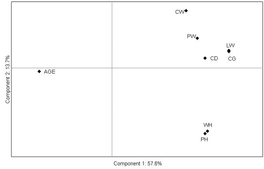
Figure 1: Projection of the morphometric measurements in the plane defined by the first two principal components. Live weight (LW); chest depth (CD); chest girth (CG); chest width (CW); pelvis width (PW); withers height (WH); and pelvis height (PH).

The coordinates of the eight initial variables in the plane formed by the axes representing the two principal components show their correlations with components 1 and 2. Component 1 showed high positive correlations with the live weight (LW), the chest width (CW), the pelvis width (PW), and the chest girth (CG), but a negative correlation with the withers height (WH) of the live animal. In fact, these variables are located far from the origin of the first component (PC1). The shape characteristics are grouped together, placed to the right of the loading plot and positively correlated. The second component (PC2) is characterized by two frame size measurements (withers and pelvis heights). In fact, the second component showed high negative correlations with withers(WH), and pelvis heights (PH), but a positive correlation with the depth of the chest (CD). In addition, these measurements are negatively correlated with the age as this parameter was located opposite to them. Hence, the principal component analysis reflected two different groups of variables. The first principal component was correlated with variables related to width and depth, indicating the animal conformation. In contrast, the second principal component was correlated to heights showing that frame size can be considered as an indicator of the axis of the animal bone structure.

Cluster analysis based on the two previously revealed components identified three classes of live cull cows (Figure 2) that could be described as follows:

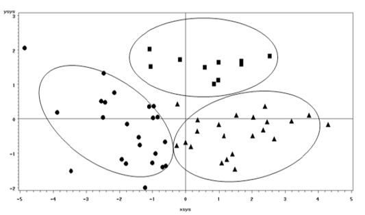
Figure 2:Projection of the morphometric measurements of the three animal groups identified by the cluster analysis based on the two principal components. : Cluster 1, : Cluster 2, : Cluster 3.

Table 3: Means of different measurements among the three classes of cull cows.

Means and standard errors of different measurements are shown in Table 3. Significant differences were found among the three live cattle clusters for all parameters measured before the slaughter (p<0.05).

These results showed that cull cows identified in cluster 2 and 3 recorded the highest live weight (LW) and chest girth (CG) compared to cluster 1 (540 kg vs. 539 and 437 kg). Vestergaard et al. (2007) reported that live weight (LW) increased simultaneously with the increase of the score of conformation of Holstein cull cows. This trend is similar to the one found in the present study. Cull cows identified in cluster 2 showed the highest withers (WH) (143 cm vs. 134 and 135 cm) and pelvis heights (PH) (146 cm vs. 138 and 137 cm) compared to cluster 1 and 3. We also revealed significant difference (p<0.05) for age between the three clusters. Culls cows identified in cluster 1 had the highest recorded age at slaughter compared to clusters 2 and 3 (9.7 years vs. 8.4 and 8.9). In addition, the cull cows grouped in cluster 1 showed the lowest values for the weight (437 kg vs. 539 and 540 kg), girth of the chest (CG) (176 cm vs. 190 cm), and depth of the chest (CD) (72 cm vs. 78 and 77cm) as well as width of the chest (CW) (38 cm vs. 40 and 42cm) and pelvis (PW) (43 cm vs. 49 and 50 cm) compared to clusters 2 and 3. Gallo et al. (2017) studied the breed effect on body traits in cull cows and found lower scores for body condition and fleshiness and had greater body measurements for specialized dairy breeds. These authors showed also that live weight and body measurement (height at withers (WH) and chest girth (CG)) increased with the increasing age in cull cows aged between 5 to 6 years at slaughter. The disparities between the results observed by Gallo et al. (2017) and the results found in the present study can be explained by the differences in age between cull cows used in our study. Cull cows in the present study were older than those used by these authors. In another study, Otto et al. (1991) reported that Holstein cull cows recorded higher body score condition in younger cows. They also showed that live weight decreased as age increased in Holstein cull cows slaughtered at different ages. These results are quite similar to those found in the present study. Shemeis et al. (1994) reported that cull cows with the lowest body condition score of their three groups also had the lowest conformation score, as was seen in the current study. In another study, Minchin et al. (2010) reported that the body condition score of Holstein cull cows improves with increased weight at slaughter, again consistent with the present study.

This study revealed the potential benefits of morphometric measurements in the assessment and qualification of live cull cows between 6 and 13 years. Principal components analysis allowed for the identification of two groups of components and the distinction between the different classes of cull cows. Cluster analysis divided the cull cows slaughtered in Tunisia into three different groups. These results might allow the use of the live weight and the pelvis height to create a classification scheme that could serve as a basis for providing information to livestock and meat operators to improve live cattle prices at the livestock auctions.

This research was conducted in cooperation with the Société Viandes du Cap-Bon. The authors are particularly grateful to this company for its technical support and assistance in collecting data. We also wish to thank Professor Joe M.Regenstein in the Department of Food Science at Cornell University for his editorial assistance.

All authors contributed equally.

The authors have declared no conflict of interest.