Prediction of Selected Reproductive Traits of Indigenous Harnai Sheep under the Farm Management System via various Data Mining Algorithms

Daniel Zaborski,1,* Muhammad Ali,2 Ecevit Eyduran,3 Wilhelm Grzesiak,1 Mohammad Masood Tariq,2 Ferhat Abbas,2 Abdul Waheed4 and Cem Tirink5

1Laboratory of Biostatistics, Department of Ruminants Science, West Pomeranian University of Technology, Szczecin, Doktora Judyma 10, 71-466 Szczecin, Poland

2Center for Advanced Studies in Vaccinology and Biotechnology, University of Balochistan, Quetta, Balochistan, Pakistan

3Department of Animal Science, Igdir University, Igdir, Turkey

4Faculty of Veterinary Sciences, Bahauddin Zakariya University, Multan, Pakistan

5Department of Animal Science, Ondokuz Mayis University, Samsun, Turkey

ABSTRACT

In this study, an attempt was made at predicting the values of selected reproductive parameters in Harnai sheep using different data mining algorithms (artificial neural networks - ANN, classification and regression trees - CART, chi-square automatic interaction detector - CHAID and multivariate adaptive regression splines - MARS) and indicating the most influential predictors of these traits. A total of 382 reproduction records including three predictors (month of lambing - MOL, age at first lambing - AFL and lambing weight - LW) and seven dependent (output) variables (services per conception - SPC, service period - SP, lambing interval - LI, twinning rate - TR, gestation length - GL, breeding efficiency - BE and fertility rate - FR) were used. A 10-fold cross-validation was applied to train and evaluate the models. The highest correlation coefficients (r) were found for LI (0.18 - 0.29; P≤0.001), GL (0.05 - 0.21; P≤0.001 to P>0.05) and FR (0.11 - 0.26; P≤0.001 to P≤0.05). For the remaining output variables, it was usually lower than 0.10. The smallest values of SDratio (0.96 - 1.06) were found for LI, GL and FR. For the rest of the output variables, it was usually above 1.00. The measures of predictor importance to ANN, CART, CHAID and MARS were generally low. In conclusion, the applied method of reproductive parameters prediction was rather ineffective, indicating that more powerful input variables are required to obtain better prediction results.

Article Information

Received 17 July 2017

Revised 30 August 2017

Accepted 13 November 2017

Available online 25 January 2019

Authors’ Contribution

MA and EE conceived and designed the study and revised the manuscript for important intellectual content. AW, MMT and FA wrote the article. DZ and WG analyzed the data. CT helped in the acquisition of data.

Key words

Reproductive traits, Harnai sheep, Artificial neural networks, Data mining, Multivariate adaptive regression splines.

DOI: http://dx.doi.org/10.17582/journal.pjz/2019.51.2.421.431

* Corresponding author: daniel.zaborski@zut.edu.pl

0030-9923/2019/0002-0421 $ 9.00/0

Copyright 2019 Zoological Society of Pakistan

Introduction

Harnai sheep is one of the indigenous breeds of Pakistan. It is a fat tail mutton and wool type breed kept mainly in the Balochistan province and characterized by a medium-sized body, white coat and black or tan spotted head and ears (Bukhari et al., 2016). In general, sheep production is one of the crucial fields of the agricultural sector in Pakistan (Tehmina et al., 2014; Safi et al., 2017) and Harnai sheep is of significant importance to the farmer community in the Balochistan province (Tariq et al., 2012). The gain or profit obtained by a farmer depends on the reproductive and productive performance of the sheep breeds being kept (Hanford et al., 2002; Zubair et al., 2006). Moreover, the differences in this performance are also caused by the exact location and the management system being used (Bukhari et al., 2016). In addition, reproduction is affected by several characteristics of ewes, such as: puberty, pregnancy, lambing, milk yield, and mothering ability. These, in turn, are influenced by genetic and environmental factors. It is very desirable in the breeding practice to be able to predict the values of economically significant reproductive traits. Such predictions can be utilized as an aid to a farmer in the decision process regarding herd management.

One way of generating such predictions is the use of statistical methods, especially those from the field of data mining. These methods include, among others, artificial neural networks (ANN), decision trees and multivariate adaptive regression splines (MARS). ANN are information processing systems based on the structure and functioning of the biological nervous system, especially of the human brain. Decision trees are the structures consisting of nodes (including a root node and leaf nodes) connected together with branches and generated using the “divide-and-conquer” strategy. They represent a set of “if-then” rules that reflect relationships between explanatory (predictor) variables and are relatively easily interpretable. Finally, MARS belongs to non-parametric regression methods, which operate locally and use the so-called spline functions to construct the complete model. More detailed information on the properties of the above-mentioned methods can be found in Grzesiak and Zaborski (2012).

Therefore, the aim of the present study was the prediction of selected reproductive traits of Harnai sheep using several data mining algorithms and the indication of the most influential predictors of these traits.

 

Table I.- Descriptive statistics for the investigated continuous variables (n=382).

Variable*	Mean±SD
AFL (days)	573.20±113.52
LW (kg)	41.80±6.85
SPC (number)	1.16±0.37
SP (days)	213.74±11.19
LI (days)	264.23±44.60
TR (%)	3.67±0.24
GL (days)	160.60±15.29
BE (%)	75.71±2.77
FR (%)	81.68±7.01

*Variable abbreviations are given in the materials and methods section.

 

Materials and Methods

The dataset

In the present study, a total of 382 reproduction records of Harnai sheep were used in the analysis. Each record consisted of one nominal and two numerical predictors and seven numerical output variables. The predictors were as follows: X1 – MOL - month of lambing (March, April, November and December), X2 – AFL - age at first lambing (days) and X3 - LW - lambing weight (kg), whereas the output variables included: Y1 – SPC - number of services per conception, Y2 – SP - service period (days), Y3 – LI - lambing interval (days), Y4 – TR - twinning rate (%), Y5 – GL - gestation length (days), Y6 – BE - breeding efficiency (%) and Y7 – FR - fertility rate (%). The descriptive statistics for the numeric variables are given in Table I. The distribution of the categorical predictor is presented in Table II.

 

Table II.- Distribution of the month of lambing (MOL).

Month	n	%
March (3)	59	15.45
April (4)	75	19.63
November (11)	133	34.82
December (12)	115	30.10

 

Statistical models

In order to prepare the models and objectively verify their predictive performance, a 10-fold cross-validation was used due to the sample size (382 cases). The following models were used for prediction: artificial neural networks (ANN), including linear networks (LN), multilayer perceptrons with one (MLP1) and two (MLP2) hidden layers and radial basis function (RBF) networks, decision trees, including classification and regression trees (CART) (Breiman et al., 1984) and chi-square automatic interaction detector (CHAID) (Kass, 1980) as well as multivariate adaptive regression splines (MARS) (Friedman, 1991).

Pseudoinversion was employed for the training of LN. In the case of MLP, a traditional error back-propagation algorithm (Rumelhart et al., 1986) was applied as a basic method of learning. Additionally, a conjugate gradient algorithm was used if necessary. In the case of the RBF networks, the centers of the basis functions were determined with the k-means method and their deviations with a k-nearest neighbor algorithm. The training of the output layer was carried out using pseudoinversion (StatSoft, 1998). All the ANN types in the present study were trained with the appropriate algorithms until reaching the lowest possible root-mean-square error (RMSE) on the validation set – a part of the learning set used for preventing overtraining. The design of the optimal networks topology and their training were performed using the Statistica Neural Networks program (v. 4.0F, StatSoft Inc., Tulsa, OK, USA). This program enabled an automatic selection of the network with the best architecture and prediction performance through the application of appropriate training parameters (the number of neurons in the hidden layers, the form of activation functions in individual network layers, the type of learning algorithm, the number of training epochs, the values of learning rate and momentum, etc.).

In the construction of the CART model, the minimum number of cases in a node was 39 and pruning was based on the variance of cases in a node, whereas when building the CHAID trees, the minimum number of cases in a node was the same as for CART, and the Bonferroni adjusted p-values for splitting and merging the categories of predictors were equal to 0.05. Moreover, the exhaustive search mode of the CHAID algorithm was used to obtain a tree with better performance.

Finally, the following MARS model was applied in the current study (Zhou and Leung, 2007):

Where, ŷ is the predicted value of the dependent variable, β0 is a constant, βm is the coefficient, hkm(Xv(k,m)) is the basis function, in which v(k,m) is an index of the predictor used in the mth component of the kth product, Km is the parameter limiting the order of interaction.

The maximum number of basis functions in the current analysis was 300 and the six-order interactions were allowed. After building the most complex MARS model, the basis functions that did not contribute much to the quality of the model performance were removed in the process of the so-called pruning based on the following generalized cross-validation error (GCV) (Koronacki and Ćwik, 2005):

Where, n is the number of training cases, yi is the observed value of the dependent variable, ŷi is the predicted value of the dependent variable, M(λ) is the penalty function for the complexity of the model containing λ terms.

The model with the smallest GCV was considered as the best one.

Goodness-of-fit criteria

The quality of all the models in the study was evaluated using the following criteria calculated as a result of the 10-fold cross-validation (Akaike, 1973; Sugiura, 1978; Salehi et al., 1998; StatSoft, 1998; Willmott and Matsuura, 2005; Takma et al., 2012; Zhang and Goh, 2016; Koc et al., 2017).

Pearson correlation coefficient (r) between the actual (observed) and predicted values

Akaike information criterion (AIC)

, if n/k>40, or

, otherwise

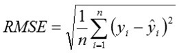
Root-mean-square error (RMSE)

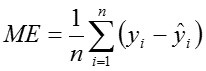
Mean error (ME)

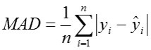
Mean absolute deviation (MAD)

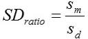
Standard deviation ratio (SDratio)

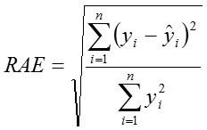
Global relative approximation error (RAE)

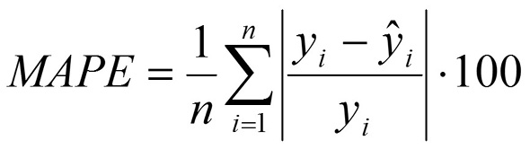
Mean absolute percentage error (MAPE)

Performance index

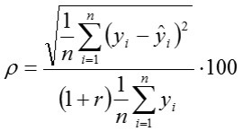
Where, n is the number of cases in a data set, k is the number of model parameters, yi is the real value of the dependent variable, ŷi is the predicted value of the dependent variable, sm is the standard deviation of the model errors, sd is the standard deviation of the dependent variable.

 

After performing the 10-fold cross-validation for each model type, the AIC values were calculated for each of the 10 models run on the whole dataset of 382 cases. The average model architecture was constructed based on the lowest AIC value obtained on this set.

Predictor importance

Finally, in order to find the most influential predictors of the reproduction parameters (seven output variables) evaluated in the present study, the error value and error ratio were used for ANN and the values obtained from the so-called importance analysis of decision trees were applied. The number of references (NoR) to each predictor was used to reveal the most influential variables for MARS. The above mentioned values were averaged over ten iterations of the cross-validation procedure and ranks were assigned on the basis of these averaged values (Eyduran et al., 2017). They are presented in Table V. Apart form ANN, all the statistical computations were made using Statistica 12 software (StatSoft Inc., Tulsa, OK, USA). Statistical significance level was considered as P≤0.05.

 

Results

Model performance

The average architectures of the ANN and MARS models obtained for the 10-fold cross-validation are depicted in Table III. In the case of decision trees, the average CART models for SPC, SP, TR and BE consisted of only one node (the root node without any splits). The average tree structures for the remaining variables (LI, GL and FR) are depicted in Figure 1. Similarly, the average CHAID models for SPC, TR and BE consisted of only one node, whereas those for the rest of the output variables are presented in Figure 2. The mean predictive performance of the applied ANN, decision trees and MARS is presented in Table IV. The highest values of the correlation coefficient (r) were noted for LI (r ranging from 0.18 to 0.29; P≤0.001), GL (r ranging from 0.05 to 0.21; P≤0.001 to P>0.05) and FR (r ranging from 0.11 to 0.26; P≤0.001 to P≤0.05). For the remaining output variables, it was usually lower than 0.10. The smallest values of SDratio were found for the three above-mentioned output variables (SDratio ranging between 0.96 and 1.06). For the rest of them, it was usually greater than 1.00. As far as AIC is concerned, the best model quality was characteristic of MLP2 (TR, GL and FR), CART (SPC, LI and BE), CHAID (SPC and BE) or MARS (SP).

Predictor importance

The most significant input variables are shown in Table V. In general, the values of the error ratio for the three studied input variables were low and in some cases even fell below 1.0. Similarly, the mean importance was often equal to 0. The most significant predictors of SPC were AFL and MOL (as indicated by ANN) or LW (as indicated by MARS). The most influential predictor of SP was LW (LN, MLP1, MLP2, CHAID and MARS) or MOL (RBF). In the case of LI and TR, each of the three input variables was indicated as the most important one (depending on the classifier). For GL, MOL and LW were the most influential factors, whereas AFL and MOL had the greatest effect on BE. Finally, MOL was the most important determinant of FR (for all the classifiers investigated in the present study).

 

Table III.- Average architectures of the investigated ANN and MARS.

MLP1	MLP2	RBF	MARS
			No. of basis functions	Degree of interaction
Number of services per conception (SPC)
6-6-1	6-23-23-1	6-5-1	5	3
Service period (SP)
6-1-1	6-35-35-1	6-1-1	8	3
Lambing interval (LI)
6-2-1	6-23-10-1	6-6-1	8	2
Twining rate (TR)
6-53-1	6-23-23-1	6-1-1	0	x
Gestation length (GL)
6-3-1	6-23-9-1	6-2-1	11	3
Breeding efficiency (BE)
6-3-1	6-23-12-1	6-1-1	7	2
Fertility rate (FR)
6-15-1	6-23-10-1	6-2-1	3	2

MLP1, multilayer perceptron with one hidden layer; MLP2, multilayer perceptron with two hidden layers; RBF, radial basis function network; MARS, multivariate adaptive regression splines.

 

Table IV.- Predictive performance of the applied models.

Measure	Unit	LN	MLP1	MLP2	RBF	CART	CHAID	MARS
No. of services per conception (SPC)
r		0.03	-0.05	-0.05	-0.06	-0.16**	-0.16**	0.00
AIC		-739.47	440.71	-486.51	-686.37	-751.04	-751.04	-722.93
RMSE		0.37	0.39	0.39	0.38	0.37	0.37	0.38
ME		0.01	-0.01	-0.01	0.00	0.00	0.00	0.00
MAD		0.27	0.29	0.29	0.28	0.28	0.28	0.28
SDratio		1.00	1.06	1.06	1.02	1.00	1.00	1.03
RAE		0.31	0.32	0.32	0.31	0.30	0.30	0.31
MAPE	%	20.12	21.87	21.92	20.79	20.72	20.72	20.96
ρ	%	30.84	35.24	35.24	34.70	37.81	37.81	32.73

Service period (SP)
r		0.14**	0.09	0.07	0.11*	-0.13*	-0.04	0.12*
AIC		1853.41	2542.90	3053.47	1911.39	1849.22	1856.32	1828.29
RMSE	Day	11.11	11.44	11.34	11.18	11.19	11.30	11.58
ME	Day	0.11	-0.55	-0.47	0.06	0.00	0.03	0.08
MAD	Day	5.44	5.30	5.05	5.22	4.95	5.05	5.25
SDratio		0.99	1.02	1.01	1.00	1.00	1.01	1.04
RAE		0.05	0.05	0.05	0.05	0.05	0.05	0.05
MAPE	%	2.84	2.79	2.67	2.75	2.63	2.68	2.75
ρ	%	4.56	4.91	4.96	4.71	6.02	5.51	4.84
Lambing interval (LI)
r		0.27***	0.28***	0.18***	0.29***	0.24***	0.21***	0.23***
Measure	Unit	LN	MLP1	MLP2	RBF	CART	CHAID	MARS
AIC		2888.14	3467.88	3418.16	2971.22	2873.46	2893.83	2964.82
RMSE	Day	43.03	43.11	44.58	43.00	42.55	43.58	46.31
ME	Day	0.96	-0.73	0.15	0.01	-0.42	0.01	0.42
MAD	Day	36.10	35.03	37.07	34.92	35.64	36.76	35.37
SDratio		0.97	0.97	1.00	0.97	0.97	0.98	1.04
RAE		0.16	0.16	0.17	0.16	0.16	0.16	0.17
MAPE	%	15.46	15.10	15.89	15.03	15.33	15.82	15.10
ρ	%	12.82	12.75	14.30	12.62	12.99	13.63	14.20
Twinning rate (TR)
r		-0.10*	-0.05	-0.05	0.05	-0.16**	-0.16**	-0.01
AIC		-1074.26	-1610.36	-2171.97	-1007.28	-1095.24	-1095.24	-1046.85
RMSE	%	0.24	0.25	0.25	0.24	0.24	0.24	0.25
ME	%	-0.01	0.00	0.00	0.01	0.00	0.00	0.00
MAD	%	0.18	0.19	0.18	0.18	0.18	0.18	0.19
SDratio		1.02	1.07	1.04	1.01	1.00	1.00	1.06
RAE		0.07	0.07	0.07	0.06	0.06	0.06	0.07
MAPE	%	5.00	5.19	4.97	4.94	4.92	4.92	5.16
ρ	%	7.26	7.16	7.16	6.22	7.78	7.78	6.90
Gestation length (GL)
r		0.13*	0.13**	0.14**	0.19***	0.05	0.05	0.21***
AIC		2096.06	2588.38	-1127.57	2154.32	2089.03	2087.07	2167.80
RMSE	Day	15.26	15.52	15.36	15.02	15.32	15.28	16.17
ME	Day	-0.21	-0.43	-0.13	0.12	-0.15	-0.01	0.41
MAD	Day	13.50	13.34	13.31	13.12	13.70	13.76	12.96
SDratio		1.00	1.02	1.01	0.98	1.00	1.00	1.06
RAE		0.09	0.10	0.10	0.09	0.09	0.09	0.10
MAPE	%	8.52	8.46	8.41	8.28	8.65	8.68	8.19
ρ	%	8.41	8.55	8.39	7.86	9.09	9.06	8.32
Breeding efficiency (BE)
r		-0.02	0.04	0.02	0.13*	-0.11*	-0.11*	0.19***
AIC		803.77	1385.32	4217.50	851.71	783.84	783.84	813.46
RMSE	%	2.81	2.86	2.84	2.76	2.78	2.78	2.78
ME	%	0.02	0.02	-0.03	-0.03	0.00	0.00	0.02
MAD	%	2.21	2.21	2.21	2.16	2.18	2.18	2.17
SDratio		1.01	1.03	1.03	1.00	1.00	1.00	1.00
RAE		0.04	0.04	0.04	0.04	0.04	0.04	0.04
MAPE	%	2.93	2.94	2.94	2.87	2.90	2.90	2.87
ρ	%	3.79	3.63	3.68	3.23	4.13	4.13	3.08
Fertility rate (FR)
r		0.26***	0.19***	0.19***	0.24***	0.11*	0.26***	0.22***
AIC		1475.86	2380.57	974.47	1526.60	1487.26	1465.77	1473.69
RMSE	%	6.78	7.10	7.01	6.83	6.97	6.76	6.88
ME	%	-0.07	0.03	-0.03	0.11	-0.01	0.00	-0.03
MAD	%	5.23	5.51	5.46	5.26	5.40	5.18	5.40
SDratio		0.97	1.01	1.00	0.97	0.99	0.96	0.98
RAE		0.08	0.09	0.09	0.08	0.09	0.08	0.08
MAPE	%	6.56	6.90	6.85	6.59	6.80	6.51	6.77
ρ	%	6.59	7.30	7.21	6.74	7.69	6.57	6.90

*, **, ***, statistical significance at P≤0.05, P≤0.01 and P≤0.001, respectively; LN, linear network; MLP1, multilayer perceptron with one hidden layer; MLP2, multilayer perceptron with two hidden layers; RBF, radial basis function network; CART, classification and regression trees; CHAID, chi-square automatic interaction detector; MARS, multivariate adaptive regression splines; r, Pearson correlation coefficient; AIC, Akaike information criterion; RMSE, root-mean-square error; ME, mean error; MAD, mean absolute deviation; SDratio, standard deviation ratio; RAE, global relative approximation error; MAPE, mean absolute percentage error; ρ, performance index.

 

Table V.- The most significant input variables for individual models.

AFL, age at first lambing; LW, lambing weight; MOL, Month of lambing; NOR, number of references.

For other abbreviations, see Table IV.

 

Discussion

As also seen from the values of the correlation coefficient, the performance of the applied models, i.e. ANN, decision trees and MARS, was very poor for all the investigated output variables. The second most important measure of predictive abilities, i.e. SDratio, also testified to the very low quality of the constructed neural and tree models as well as MARS. This result was mainly caused by the weak predictors of the reproductive parameters used in the present study. MOL, AFL and LW turned out to be insufficient for the accurate estimation of the future values of the reproductive traits analyzed in the present work. In the study by Texeira et al. (2008) on the effect of environmental factors (i.e. forage availability and climatic conditions) on the mean number of lambs per ewe (marking rate) in Patagonia, the best multiple linear regression model including predictors such as the month of growing season start and the normalized difference vegetation index in May was characterized by a relatively low predictive power (prediction determination coefficient equal to 0.14) similarly as in the present work. However, the ANN (in the form of MLP1) used for the same purpose had much better predictive performance (prediction determination coefficient equal to 0.64). Moreover, the authors of the cited study analyzed the ability of multiple regression and ANN to correctly predict the category of the year (above, below or within 5% of an average normalized marking rate). The percentage of correct indications in this analysis was 40.6% and 84.4% for the multiple linear regression and ANN, respectively. In another study (Piwczyński, 2009) on the application of classification trees to the analysis of discrete reproductive traits in 6,586 Polish Merino sheep, the most influential factors affecting the number of offspring reared until 100 days of age by a mated ewe (reproductive performance index) were ewe’s age at lambing, flock, body weight at 12 months of age and birth type (singleton vs. twins). The author concluded that the best results of reproductive performance were recorded for the ewes from twin litters, weighing at least 48.5 kg at the age of 12 months and being at least 4 years old at lambing. However, the predictive abilities of the applied decision tree model (such as a percentage of correctly classified cases) were not reported in the cited study.

In contrast, such information was provided by Olesen et al. (1994), who used linear, threshold and Poisson models for analyzing the number of lambs born by 1-year-old ewes based on the flock-year and sire effects in two Norwegian sheep breeds (Dala and Spaelsau). The mean squared error ranged from 0.25 to 0.26 depending on the model type and breed, whereas the Pearson correlation coefficients between observed and predicted values ranged from 0.26 to 0.28. So, they were comparable to the highest values of the correlation coefficient obtained in the present work.

The next study (Matos et al., 1997) on the use of different statistical models (linear, threshold, Poisson and negative binomial sire models, as well as linear, threshold, Poisson and negative binomial animal models) for reproductive traits prediction (fertility, litter size and ovulation rate) in Rambouillet and Finnsheep sheep revealed their moderate predictive performance. The models of fertility included the effects of year, body condition score at breeding and age, whereas those for the litter size and ovulation rate contained breeding weight instead of a condition score. The mean squared error for fertility ranged from 0.13 to 0.14 depending on the model type and breed with the Pearson correlation coefficient between observed and predicted values ranging from 0.18 to 0.21. The mean squared error for the litter size ranged between 0.24 and 0.39 with the correlation coefficient ranging from 0.37 to 0.47, whereas the mean squared error for the ovulation rate (only for the Rambouillet sheep) amounted to 0.31 – 0.33 with the correlation coefficient ranging between 0.38 and 0.45. The above-mentioned values were obtained for the models including permanent environmental effects. Somewhat worse results in terms of predictive abilities were recorded in the cited study for the linear and threshold models without these effects. In a similar work (Casellas et al., 2007) on the litter size and days to lambing in 376 Ripollesa ewes using univariate and bivariate threshold-linear and linear-linear models (including ewe age, lambing year and the permanent environmental effect of the ewe), the predictive ability expressed as a mean squared error and correlation coefficient between observed and predicted values was also moderate (the former ranging from 0.23 to 0.24 for the litter size and from 203 to 209 for the days to lambing and the latter ranging between 0.47 and 0.54 for the litter size and between 0.53 and 0.54 for the days to lambing, depending on the model type). However, in general, the results reported by the authors of the last two articles were relatively better than those obtained in the present work.

As far as the predictors of the individual reproductive traits are concerned, it should be clearly stated that their overall effect on the values of these parameters was rather small, which resulted in the low predictive performance of the generated models. However, their relative importance to the models predicting seven reproductive traits analyzed in the present study can be indicated. And so, month of lambing (MOL) was the most influential for SPC, SP, TR, LI, GL, BE and FR (depending on the model type). Pollott and Gootwine (2004) declared that the month of lambing and an interaction between farm and month as well as farm and month and year significantly affected LI in Assaf sheep. Also, lambing season (wet or dry) significantly affected LI in Black, White and Brown West African Dwarf sheep (Fadare, 2015). LI was shorter for the ewes lambing in the wet season (7.8 months on average) compared with that for the ewes lambing in the dry season (8.0 months on average). In Lohi sheep, Babar and Javed (2009) found that lambing season significantly affected SPC. It was higher (1.37 on average) in ewes bred in autumn than in those bred in spring (1.16 on average). However, according to Jahan et al. (2013), lambing season (spring, autumn) did not influence traits such as: fertility, twinning rate and prolificacy in Balochi sheep in Pakistan. Similar results were obtained by Ashebir et al. (2016) in Begayt sheep in Ethiopia. On the other hand, Gbangboche et al. (2006) showed that litter size in Djallonke sheep was slightly higher in the rainy season and lower in the dry one.

The next predictor (AFL) investigated in the present study was the most influential for SPC, LI, TR, and BE (depending on the model type). Babar and Javed (2009) reported that age at lambing significantly affected SPC in Lohi sheep (the higher the ewe age, the higher the SPC). According to the cited authors, younger ewes required 1.18 services per conception on average, whereas older ones took 1.34 services per conception on average. In the study by Boujenane et al. (2013), age at lambing significantly affected conception rate with the higher values (0.96 - 0.97) observed for the ewes lambing at less than 1.5 years of age and between 2.0 and 3.0 years of age, and the lower values (0.91 - 0.93) for the remaining ewes (age of lambing between 1.5 and 2.0 years and above 3.0 years). However, Ashebir et al. (2016) found a non-significant effect of ewe age on LI in Begayt sheep. The last input variable analyzed in our study (LW) was the most important predictor for SPC, SP, LI, TR and GL. A significant effect of LW on LI observed in the present work was confirmed by Gbangboche et al. (2006), who informed that heavier Begayt ewes in live body weight had shorter lambing intervals.

 

Conclusions

The proposed method of reproductive parameters prediction applied in the present study was rather ineffective, mainly due to the use of weak predictors. An application of more appropriate input variables would be required in order to obtain better prediction results.

 

Statement of conflict of interest

The authors declare that there is no conflict of interests regarding the publication of this article.

 

References

Akaike, H., 1973. Information theory and an extension of the maximum likelihood principle. In: Second International Symposium on Information Theory. Akademiai Kiado, Budapest, Hungary, pp. 267-281.

Ashebir, G., Haile, G.N. and Weldu, K., 2016. Reproductive performance of Begayt sheep under different management systems in Western Zone of Tigray. J. Dairy Vet. Anim. Res., 3: 1-5. https://doi.org/10.15406/jdvar.2016.03.00077

Babar, M.E. and Javed, K., 2009. Non-genetic factors affecting reproductive traits in Lohi sheep. Acta Agric. Scand. Sect. A, 59: 48-52. https://doi.org/10.1080/09064700802650035

Boujenane, I., Chikhi, A., Sylla, M. and Ibnelbachyr, M., 2013. Estimation of genetic parameters and genetic gains for reproductive traits and body weight of D’man ewes. Small Rumin. Res., 113: 40-46. https://doi.org/10.1016/j.smallrumres.2013.02.009

Breiman, L., Friedman, J., Stone, C.J. and Olshen, R.A., 1984. Classification and regression trees. CRC Press, Boca Raton, FL, USA.

Bukhari, F.A., Ahmad, S., Islam, M., Asmat, T.M., Rafique, M., Hameed, T., Mustafa, M.Z., Abbasi, B.H. and Ali, I., 2016. Wool production performance of Harnai sheep from Asghara valley, Sinjavi, District Ziarat. Pure appl. Biol., 5: 1.

Casellas, J., Caja, G., Ferret, A. and Piedrafita, J., 2007. Analysis of litter size and days to lambing in the Ripollesa ewe. I. Comparison of models with linear and threshold approaches. J. Anim. Sci., 85: 618-624. https://doi.org/10.2527/jas.2006-365

Eyduran, E., Zaborski, D., Waheed, A., Celik, S., Karadas, K. and Grzesiak, W., 2017. Comparison of the predictive capabilities of several data mining algorithms and multiple linear regression in the prediction of body weight by means of body measurements in the indigenous Beetal Goat of Pakistan. Pakistan J. Zool., 49: 257-265. https://doi.org/10.17582/journal.pjz/2017.49.1.257.265

Fadare, A.O., 2015. Reproductive traits among Black, White and Brown West African Dwarf sheep. Livest. Res. Rural Dev., 27: 24.

Friedman, J.H., 1991. Multivariate adaptive regression splines. Annls. Stat., 19: 1-67. https://doi.org/10.1214/aos/1176347963

Gbangboche, A.B., Adamou-Ndiaye, M., Youssao, A.K.I., Farnir, F., Detilleux, J., Abiola, F.A. and Leroy, P.L., 2006. Non-genetic factors affecting the reproduction performance, lamb growth and productivity indices of Djallonke sheep. Small Rumin. Res., 64: 133-142. https://doi.org/10.1016/j.smallrumres.2005.04.006

Grzesiak, W. and Zaborski, D., 2012. Examples of the use of data mining methods in animal breeding. In: Data mining applications in engineering and medicine (ed. A Karahoca). InTech, Rijeka, Croatia, pp. 303-324. https://doi.org/10.5772/50893

Hanford, K.J., Van Vleck, L.D. and Snowder, G.D., 2002. Estimates of genetic parameters and genetic change for reproduction, weight, and wool characteristics of Columbia sheep. J. Anim. Sci., 80: 3086-3098. https://doi.org/10.2527/2002.80123086x

Jahan, M., Tariq, M.M., Kakar, M.A. and Waheed, A., 2013. Reproductive performance of Balochi sheep in different ecological zones of Balochistan, Pakistan. Pak. Vet. J., 33: 37-40.

Kass, G.V., 1980. An exploratory technique for investigating large quantities of categorical data. J. R. Stat. Soc. Ser. C Appl. Stat., 29: 119-127. https://doi.org/10.2307/2986296

Koc, Y., Eyduran, E. and Akbulut, O., 2017. Application of regression tree method for different data from animal science. Pakistan J. Zool., 49: 599-607. https://doi.org/10.17582/journal.pjz/2017.49.2.599.607

Koronacki, J. and Ćwik, J., 2005. Statistical learning systems. WNT, Warsaw, Poland.

Matos, C.A., Thomas, D.L., Gianola, D., Perez-Enciso, M. and Young, L.D., 1997. Genetic analysis of discrete reproductive traits in sheep using linear and nonlinear models: II. Goodness of fit and predictive ability. J. Anim. Sci., 75: 88-94. https://doi.org/10.2527/1997.75188x

Olesen, I., Perez-Enciso, M., Gianola, D. and Thomas, D.L., 1994. A comparison of normal and nonnormal mixed models for number of lambs born in Norwegian sheep. J. Anim. Sci., 72: 1166-1173. https://doi.org/10.2527/1994.7251166x

Piwczyński, D., 2009. Using classification trees in statistical analysis of discrete sheep reproduction traits. J. Cent. Eur. Agric., 10: 303-309.

Pollott, G.E. and Gootwine, E., 2004. Reproductive performance and milk production of Assaf sheep in an intensive management system. J. Dairy Sci., 87: 3690-3703.

Rumelhart, D.E., Hinton, G.E. and Williams, R.J., 1986. Learning representations by back-propagating errors. Nature, 323: 533-536. https://doi.org/10.1038/323533a0

Safi, A., Kaleri, H., Muhammad, G., Kaleri, R., Kaleri, A., Safi, M., Ullah, A., Mandokhial, K. and Siddiq, M., 2017. Effect of genetic parameters on some growth performance traits of Harnai sheep. J. Basic appl. Sci., 13: 60-62. https://doi.org/10.6000/1927-5129.2017.13.11

Salehi, F., Lacroix, R. and Wade, K.M., 1998. Improving dairy yield predictions through combined record classifiers and specialized artificial neural networks. Comput. Electron. Agric., 20: 199-213. https://doi.org/10.1016/S0168-1699(98)00018-0

StatSoft, 1998. Statistica Neural Networks user guide. StatSoft, Inc., Tulsa, OK, USA.

Sugiura, N., 1978. Further analysts of the data by Akaike’s information criterion and the finite corrections. Commun. Stat. Theory Methods, 7: 13-26. https://doi.org/10.1080/03610927808827599

Takma, Ç., Atil, H. and Aksakal, V., 2012. Çoklu doğrusal regresyon ve yapay sinir ağı modellerinin laktasyon süt verimlerine uyum yeteneklerinin karşılaştırılması. Kafkas Üniv. Vet. Fakül. Derg., 18: 941-944.

Tariq, M.M., Bajwa, M.A., Jawasreh, K., Awan, M.A., Abbas, F., Waheed, A., Rafeeq, M., Wadood, A., Khan, K.U., Rashid, N., Atique, M.A. and Bukhari, F.A., 2012. Characterization of four indigenous sheep breeds of Balochistan, Pakistan by random amplified polymorphic DNAs. Afr. J. Biotechnol., 11: 2581-2586. https://doi.org/10.5897/AJB11.3196

Tehmina, S., Shahina, R., Razzaq, A., Marghazani, I.B. and Khosa, A.N., 2014. Prevalence of Paramphistomum cervi in different sheep breeds of Balochistan (Pakistan). Rev. Vet., 25: 12-15.

Texeira, M., Paruelo, J.M. and Jobbagy, E., 2008. How do forage availability and climate control sheep reproductive performance?: An analysis based on artificial neural networks and remotely sensed data. Ecol. Model., 217: 197-206. https://doi.org/10.1016/j.ecolmodel.2008.06.027

Willmott, C.J. and Matsuura, K., 2005. Advantages of the mean absolute error (MAE) over the root mean square error (RMSE) in assessing average model performance. Clim. Res., 30: 79.

Zhang, W. and Goh, A.T., 2016. Multivariate adaptive regression splines and neural network models for prediction of pile drivability. Geosci. Front., 7: 45-52. https://doi.org/10.1016/j.gsf.2014.10.003

Zhou, Y. and Leung, H., 2007. Predicting object-oriented software maintainability using multivariate adaptive regression splines. J. Syst. Softw., 80: 1349-1361. https://doi.org/10.1016/j.jss.2006.10.049

Zubair, M., Habib, G. and Ahmad, N., 2006. Comparative study on wool yield and wool quality in sheep reared at Livestock Research Station Jaba and Lalazar alpine pasture. J. Anim. Vet. Adv., 5: 641-646.