Research Article

Estimating Sample Size and Fitting Multilevel Model in Agricultural Experiments

Iftikhar Ud Din* and Qamruz Zaman

University of Peshawar, Khyber Pakhtunkhwa, Pakistan.

Received | March 08, 2019; Accepted | April 20, 2019; Published | May 20, 2019

*Correspondence | Iftikhar Ud Din, University of Peshawar, Khyber Pakhtunkhwa, Pakistan; Email: iftikhar.din1@gmail.com

Citation | Din, I.U. and Q. Zaman. 2019. Estimating sample size and fitting multilevel model in agricultural experiments. Sarhad Journal of Agriculture, 35(2): 630-638.

DOI | http://dx.doi.org/10.17582/journal.sja/2019/35.2.630.638

Keywords | Multilevel modeling, Intra-class correlation, Standard error, Effect size, Power of the test

Introduction

Hierarchical or multilevel data structures have great utility in many areas of agricultural research including on-farm trials, where there can be information at the village, farm and plot or animal level. Experiments in animal breeding are often concerned with attributing variation in traits of offspring, such as their mortality, fertility rates and subsequent growth rates (Li et al., 2017). All those concerned with agricultural research are quite familiar with the phenomena that livestock data often have some hierarchical structure with different levels of variation. Analysis of variance except in balanced or nested designs has been difficult to apply to data with a multilevel structure. Mixed modelling is becoming a standard approach for analyzing these types of data, particularly since it can deal with complicated or “messy” structures (Hebblewhite, 2008).

In multilevel data structures there are different types of investigational units at different levels or layers, e.g. plots within farms, or animals within herds and attributes associated with these different units whose effects we wish to assess, e.g. planting density, thinning practice, breed or sex of the animal. The response of interest, such as crop yield or weaning weight, is usually measured at the lowest level, but the variation in these responses is due to variability at the different levels. For example, variation in crop yields collected in an on farm trial is partly due to village to village variability, farm to farm variability or partly due to plot to plot variability. To incorporate these different levels of variability into our multilevel model for hierarchical data, we specify the units in the levels as random effects.

Multilevel model (MLM) is very powerful technique and has wide range of applications (Gilbert, 2008). One strong reason for using mixed modelling is that it can deal effectively with levels or layers in the data and can give more valid, though theoretically approximate, significance tests and standard errors, something that conventional analysis of variance methods cannot do except in one or two specific circumstances. Secondly, it has the ability, with unbalanced structures, to combine information from different level in the data (Kreft and Leeuw, 1998). Readers who are familiar with the analysis of lattice designs will recognize that this is akin to “recovering inter-block information”. This has the added advantage of improving the precision of fixed effect comparisons such as the experimental treatments or other covariates. The one slight drawback of the model is that initially it seems relatively complex compared to analysis of variance. For a start, the model is more difficult to specify one needs to correctly identify which effects are random and which are fixed. The resulting computer output is also less familiar and not easy to use than ANOVA outputs. However, researchers who are familiar with split-plot analysis of variance will probably have less difficulty in formulating the multilevel model, since the principles of identifying and evaluating variation of more than one level in the data is the same. Thus, wherever, the composition of data is hierarchical in nature, we should go for the appropriate mixed model analysis (Goldstein, 2011). This study is intended to explore and understand the multilevel modeling that will lead to a better ability on the part of the reader to recognize the correct analysis-­ a step closer to the best model. Multilevel model is capable to extract interaction between level 2 and level 1, say village × field, often such interactions are of key interest (Aguinis et al., 2013). Finally, a clear awareness at the planning stage is definitely needed to ensure that how much different levels of units should be included in a proposed study and also to add sufficient replication at each level.

It is often observed in agriculture, particularly in agriculture economics and agriculture extension that sampling methodology desire the use of multistage cluster sampling. In this context sampling from certain district involve random selection of villages and from villages fields are randomly selected, similarly, sampling can be extended from two to higher stages. In such type of sampling the neighborhood effect is most likely to carry over. To capture this effect an important class of statistical modeling called multilevel modeling came into limelight, which not only investigate the individual effect but also the contextual effect as well (Goldstein, 2003; Raudenbush and Bryk, 2002; Snijders and Bosker, 1999).

Another problem which can be confronted in these situations is the dependence of the observations and consequently the violation of the assumptions commonly known as Gauss-Markov assumption (where observations are regarded as independent and identically distributed).

One of the foremost problem in handling multilevel modeling is the estimation of optimum sample size for carrying out the investigation. (Murray et al., 2006) This study is intending to investigate the problem by considering multilevel models restricted to two levels but the same reasoning can be extended to higher levels as well. At the outset we consider a basic multilevel model.

 

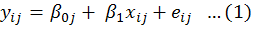
where;

which can be written more compactly.

 

where;

yij may be the yield of the ith field in the jth village randomly selected from district A. Model (1) is based on random intercept i.e. we allow intercept to vary from village to village while the slope coefficient is fixed for the villages. Here we need to estimates four parameters namely.β0, β1 and σ2e, σ2uo (Raudenbush, 2004).

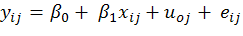
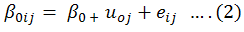
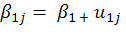
In case it is expected that the role of the covariate also changes from village to village. In a given problem this may be the fertility gradient which may change from village to village and consequently we can consider it random as well and the model (1) now becomes, (Hox, 1995).

 

 

 

For illustration, one can obtain the estimate of,

 

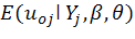
where;

 

It is evident that in model (2) there are two fixed coefficients, β0, β1 while σ2uo, σuo1, σ2u1 and σ2eo are the random parameters, σ2uo and σ2u1 are the variances associated with random intercept and random slope respectively, while σu 01 is the covariance between these terms. These variances and covariances are termed as random parameters. (Demidenko, 2013).

Sample size issue in multilevel modeling

One of the core issues in carrying multilevel modeling is estimation of sufficient sample size. Conventionally, the factors affecting sample size are the precision desired for the given type of estimate, its variability, and the types of sampling. The additional factors which are contributing in the estimation of sample size for multilevel models are intraclass correlation (ICC), the number of parameters in the model, and the balancing status of the data are vital. Generally, it is believed that multilevel modeling is a large sample activity (Snijders and Bosker, 1993).

The main concern of the present research study is:

1. 1. to assess the role of the sample size in obtaining precise estimates of the fixed and random effects for fitting linear multilevel models and to analyze their subsequent power patterns.
2. 2. to find out the effect of level 1 and level 2 units in achieving optimum sampling results.
3. 3. to investigate the situations where ignoring hierarchical data structure leads to seriously misleading conclusion.

 

Materials and Methods

The methodology adopted constitute two broad sections. One relating to optimum sample selection which includes sample size in multilevel modeling and its connected factors like ICC, test size, effect size, cluster size, power of the test and number of clusters to be sampled. The second component is relating to estimation of multilevel model.

Sample size estimation

To investigate any of the problem concerning agricultural experiments in greatly dependent on the use of appropriate statistical model. Different statistical models are used for achieving the required objectives concerned with these experiments. Of these, MLM is of great importance as compared to usual traditional methods of ANOVA (Preacher, 2010). An important problem in multilevel modeling is to estimate optimum sample size, and strive to achieve minimum variance unbiased estimates of the concerned parameters. In the uni-level modeling, the factors effecting the sample size are the standard error of the effect size, power of estimation, effect size and test size but in multilevel modeling additional factors to these, like the magnitude of the ICC, number of parameters to be estimated, cluster size, total number of clusters, and the information whether the design is balanced or unbalanced are playing vital role in the estimation of sample size (Sastry et al., 2006). The statistical significance of these factors for multilevel models are evaluated and their mutual relationship is explored. In case of linear models, all the inferences are performed under the assumption of multivariate normal distribution.

Generally, in simple case when dealing with univariate normal distribution, the following formula is considered for estimation of sample size which is extended to a wide range of situation.

 

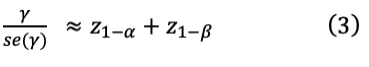
Equation (3) comprises four quantities, namely, α, the size of the test, 1-β denote the power of the test, γ is the effect size which is based on the assumption that the null hypothesis about the underlying variable has value 0, i.e. the effect size represents the increase in the parameter value. The difficulty with this expression in case of multilevel modeling is the determination of mathematical expression for se(γ). For some specific sample sizes/designs the problem can be solved using the theory of package PinT, developed by Snijders et al. (2005).

In the present research study, sample size consideration for two-factor regression and the power of estimation were observed through simulations. It is important to mention that for the regression and ANOVA type models, a specifically designed statistical package OD (Optimal Design) was used for obtaining optimum sample size for performing agricultural experiments.

Estimation of multilevel model

To achieve the data of the desired nature, simulation seems the best option. In fact, this study is continuation of our previous work (Yar et al., 2016), where students score data was taken from the schools of district Charsadda and comparison between multilevel and multiple regression analysis was made. The nutshell of the study was that it will be far convenient to compare these two models through simulations. For estimating multilevel model, data will be simulated for the yield of the crop fulfilling normality assumption. Initially considering that the yield does not change significantly from village to village, then for the intercept model, the goodness of classical linear regression model (CLRM) and multilevel linear regression (MLM) are compared. Secondly, the data is simulated such that yield does changes significantly from village to village (cluster to cluster). Again, the same comparison as stated above is made.

The process mention will be repeated using extended model, by adding covariate (Random slope in case of multilevel linear regression) to the model and the models achieved in each case will be compared for adequacy. The analysis will be carried out using nlme package of R.

Statistical analysis and discussions

Estimation of optimum sample size for multilevel modeling: Optimum sample size is estimated for different type of models. Consider a random intercept model, for illustration it is assumed that the standard error of the estimate is fixed.

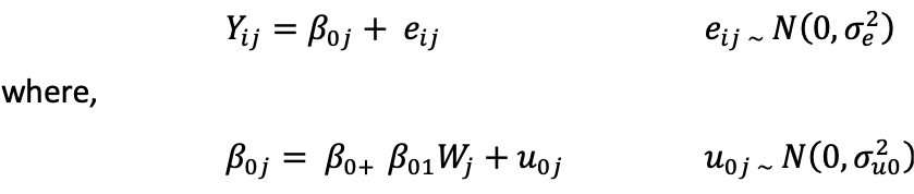
We consider the 2-level random intercept model given as (Hox, 1995).

 

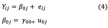
where eij ~ N (0, σe2 ) and uij ~ N (0, σu2) contain no explanatory variable.

The mixed model is:

The response Yij is a Z-score of the crop yield which is expected to vary from field to field. The response may be any continuous variable, fulfilling the assumptions (say production of crop, income or profit of farmers, net weight of animals, crop or leaf quality index etc.) and is expected to vary from field to field (level-1) and from village to village (level-2 units).

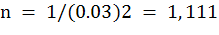
Let it is desired that within each level-2 unit (village) the mean should be estimated with a standard error of 0.03. If a simple random sample is to be taken it can readily be deduced that the sample size should be:

 

 

If a two stage sampling scheme is employed the interest will be to reassess the sample size and what will happen to the standard error if a two-stage sampling scheme is employed (first villages then fields), in case the between villages variance is 0.20, and assuming that there are direct extra budgetary consequences of sampling villages.

Case-I: when ρ = 0.1: In case intraclass correlation ρ is 0.1, then the estimated sample size in cases of two stage sampling or two level model when it is intending to brought down the standard error of the constant to 0.03 is given below. In these calculation, it was assumed that there is no extra cost involved in surveying an additional village.

In this case, ρ = 0.1. Using Cochran’s formulae and assuming that per cluster one unit will be sampled, so that n = 30, the total sample size for a two-stage random sample that is equivalent to a simple random sample (SRS) (size 1111) times design effect (3.9) that is 4333.

To maintain the standard error of 0.03, the desired sample 144 villages (J) and from each village 30 fields (n) will be selected, which makes total of 4320 fields, as given in the Supplementary Table 2 of the appendix. In these calculation the additional cost of surveying the extra cluster is taken as zero.

Case-II: when ρ = 0.2: When estimating the intercept of the multilevel model with the standard error of the estimates= 0.03. In case intra class correlation, ρ = 0.2, the desired standard error (0.03) of the estimate can be obtained using 128 villages (clusters, J) and from each 59 fields (n), this makes a total (J*n) of 7552 units. Supplementary Table 1 of the Supplementary section gives the detail situation.

Where; J, indicates the number of (villages) clusters and n, is the size of the cluster (village) and c denotes the cost per unit(field). Similarly, if it is intended to lower the standard error to 0.02, the sample size for the simple random sample (SRS) will climb to 2500 (Supplementary Table 2).

From the results of Supplementary Table 1, it is clear that there exists positive relationship between ICC and the sample size desired for the multilevel modeling. Supplementary Table 2 further authenticate the relation between standard error, ρ and their respective sample sizes.

As indicated by the output that the standard error of 0.02 can be achieved if 566 clusters each of size 30 units are surveyed. Further, it is evident that for a specified ρ, substantial reduction in the sample size and number of clusters (villages) to be sampled can be achieved if we allow the standard error to increase or add effective covariate in the model.

Two level, two factor ANOVA model

Revisit the level-1 model, the same as given in Model 1,

The level 2 model, or cluster-level model has been changed, an additional indicator variable wj is added to the model,

 

where β0 is the grand mean, β01 is the mean difference between the treatment and control group or the main effect of treatment, wj is an indicator variable taking -½ for the control group and ½ for the experimental group, u0 j is the random effect associated with each cluster, σ2uo is the variance between clusters.

The mixed model is:

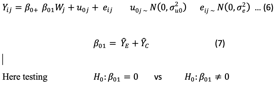
ȲE is the mean for the experimental group, ȲC is the mean for the control group.

Here testing H0 and H1 is equivalent to testing the main effect of the treatment. The problem is handled using OD (Optimal Design) for longitudinal and multilevel research. The above problem is discussed under different conditions, the main interest lies in how different factors i.e. number of clusters (J), cluster size (n), standardized effect size (δ), Intra-class correlation (ρ) and Power of the test are interacting in the precision of estimation. In particular, total sample size J × n, the product of the number of clusters sampled and the cluster size is the focal point. In order to know how cluster size and sample size varies to achieve reasonable power for managing standard estimation, α is taken as fixed at 0.05, δ at 0.20 and varying J, n, and ρ to check the power of estimation of parameters involve in two factor ANOVA model.

Sample size options when effect size is specified

The results regarding power of estimation for varying n, j, and ρ are obtained. The following outcomes are extracted from the results:

1. 1. There will be a little problem in estimation of sample size for fitting multilevel model if standardized effect size δ is 0.2 or lower and intra-class correlation ρ is also low (0.05 or less). When ρ is low, it is evident that the design effect (1+ (n-1) ρ) will be low in this case. The power, here increase rapidly with increasing number of clusters. Substantial, Power (0.80) can be achieved for J=50 or more each of size 98 (total sample size 4900). A small upward shift in the ρ (0.07), causes the total number of clusters to jump to 60 each of size 256 (total sample size 15360) for carrying a test of reasonable power (0.80) and this number rise to 85 each of size 145 (total sample size 12325) when ρ=0.10, which leads that the number of sampled clusters needed to be raised as the neighborhood effect, ρ (Intraclass correlation) increases.
2. 2. Secondly, it is observed that the cluster size is also playing a role in power enhancement, in case ρ is very small (ρ = 0.05), the influence of the cluster size diminishes when ρ increases. This can be viewed for changing the cluster size against the same cluster numbers for the respective ρs.
3. 3. From the results it is concluded that a small standardized effect size (δ = 0.20) in multilevel modeling can be detected with reasonable small samples provided that the number of clusters exceed 100. However, these options needed to be reassessed if the cost per cluster is large and the budget constraint leads the researcher to go for optimal sample size.
4. 4. It is found that generally, with the increasing number of cluster J, the cluster size n, as well as the total sample size decreases and the power of estimation is improving. For ρ = 0.05, the combination of (55, 55), (60, 40), (70, 25), (75, 20), (80, 20), (85, 14), (90, 14), (100, 13), (102, 10), (140, 8) and (160, 6), having the same power for varying number of J, n and total sample size.

 

Multilevel modeling versus classical linear regression model

The simulated data is used to fit intercept model for the crop yield in case of classical linear regression model and then allow the mean yield to change from village to village and make use random intercept model (MLM). Two sets of data are generated, the fitted models are given in Supplementary Table 3(a) of the Supplenentary Material section:

	Intercept	Residual
Std Dev	3.76	88.78

 

The low amount of standard deviation (3.76) of the intercept indicate that the crop yield does not changes markedly from village to village. Consequently, we gain nothing by using multilevel modeling approach. In fact, standard error in case of MLM is fractionally greater and t-value is low too because three parameters will be estimated in case of multilevel model.

Supplementary Table 3(b) compares the traditional linear regression model with the corresponding multilevel model on the basis of three criteria Akaike Information criteria (AIC), Bayesian Information criteria, and log likelihood function.

The Akaike’s Information and Bayesian information are fractionally larger for the MLM. As AIC penalizes MLM, for the larger the number of parameters to be estimated. In this situation, considerable high p-value refer to the suitability of classical linear regression model. The above process is repeated with another set of data, now inducing village to village variation (Standard deviation = 279.83) in the crop yield. Let’s see the output:

	Intercept	Residual
Std Dev	279.83	64.47

 

Supplementary Table 4(a) gives the coefficient of the fitted models from simulation 2, For the same mean value of the crop, MLM attribute more variation to the intercept term (88.54) with smaller degree of freedom because more parameters are estimated in case of MLM.

 

In Supplementary Table 4(b) of the Appendix, the goodness of the two models are compared, Now The MLM has now reduced the AIC and BIC by considerable margin, so is the margin between log likelihood score, consequently, the traditional and multilevel models are significantly different and the likelihood ratio test (L.Ratio) results indicates that MlM is much superior as compared to its counterpar (CLRM).

Adding covariates in the model

Lets two covariates are added to the model which are expected to be influencing the yield (response) of the crop, say the amount time spend by the farmer in the field and the amount of urea under cultivation. Now the simulated data about the crop yield, along with the two covariates reveals the following findings taken from Supplementary Table 5 in the Appendix section.

Random effect of the intercept		Intercept	Residual
	Std Dev	279.83	64.47
Random effect of the covariate	Intercept Time Residual	Std Dev 2.56e + 2 , 1.60e-04 6.42	Correlation   -0.001

 

The intercept of the constant and covariate (Time) possess high standard deviation and are highly expected to vary from village to village. In Supplementary Table 5(a) the results of the classical linear regression model and the corresponding multilevel model are given, Supplementary Table 5(a) MLM has markedly changed the status of intercept and covariate 1 coefficient. In CLRM these coefficients are insignificant while in MLM they are significant. In particular, the sign of covariate 1 coefficient also changes.

From Supplementary Table 5(b) the difference between CLRM and MLM is evident. The three criteria used namely, AIC, BIC and log likelihood showing highly significant improvement when MLM is enacted as compared to CLRM.

Supplementary Table 6(a) gives the summary of estimation when the same model is simulated once again two coefficient declared insignificant by CLRM becomes significant in MLM. Further, the sign of covariate 1 coefficient also changes.

Supplementary Table 6(b) indicates the model comparison in simulation 2. The superiority of MLM is quite evident. The corresponding likelihood ratio test shows highly significant improvement while using MLM.

Supplementary Table 7(a) gives simulation 3 history of the two models. Although the significance status of the coefficients does not change in MLM, even then the p-values declines considerably and the sign of the covariate 2 coefficient also changes.

 

From Supplementary Table 7(b) reveals the same conclusion as derived from previous two simulations. The results of these simulations are presented in the tables given in the Appendix. The likelihood test showing highly significant improvement when MLM is used instead of CLRM.

Supplementary Table 8(a) indicates that significance of two coefficients are alter when we shift from CLRM to MLM they are the intercept and the covariate 1 coefficient.

Supplementary Table 8(b) is repeating the same information by simulation 4, i.e. intra cluster variation if substantial then MLM is significantly improved model as compared to CLRM.

The extended model containing random intercept, random slope and fixed effect slope is simulated four times. The above results show that applying traditional modeling approach and ignoring village (cluster or group) effect may be seriously misleading. The analysis indicates that we may face all sorts of problem in the model, ranging from change in the size and sign of the regression coefficient(s) to the overall goodness of the model. Model comparison from all the four simulation indicate considerable higher value from likelihood ratio (L. Ratio) test which reflect highly significant difference when we shift from classical approach to the multilevel modeling approach under the conditions that between clusters (villages) variations are substantial. Significant changes are observed in the all the three criteria used for the best model selection, namely, Akaike information, Bayesian information criterion and log likelihood criteria.

Conclusions and Recommendations

From the above discussion, it came to the knowledge that sample size estimation in multilevel modeling is a complex issue, as many factors are interplaying and each has a role to play in the process. However, after thorough assessment of the factors involved in estimation of sample size for multilevel modeling, we conclude with the following points.

1. 1. In agricultural trials, one of the major components in the sample size estimation is intra- class correlation i.e. correlation between fields, villages, tehsils and districts etc. This causes the sample size to rise sharply. It is observed that an intra-class correlation of small amount (say 0.1) inflates the sample size to almost 4 times as compared to simple random sampling. However, it is recorded that equal increment in ICC does not change the sample size uniformly i.e. its effect reduces slowly as ICC is increasing.
2. 2. There are variety of choices available for the researchers, with multistage sample having the same power status, which can suits the study if the resources permits. For example, when ρ = 0.05, all combinations of J and n given by (35, 6), (50, 4), (65, 3), (70, 3), (85, 2), (100, 2) which makes total sample (J×n) of considerable small size, possess sufficient power for estimation and are in contention, if the cost incurred in observing additional cluster is not creating problem. If this is not the case, then naturally option one (35, 6) seems to be a better choice. This conclusion is supported by McNeish and Stapleton (2016) that is to effectively utilize multilevel models, one must have an adequately large number of clusters; otherwise, some model parameters will be estimated with bias.
3. 3. In agricultural experiments conducted at different locations, in field trials experiments, the observations are often effected by the neighbourhood or environmental effect which may vary from small to large in magnitude. This effect is needed to be captured in the statistical model and ignoring such effect by considering observations to be independently distributed may leads to serious consequences ranges from misleading conclusion to the lack of model adequacy. In case of no or negligible effect, ignoring village (cluster) effect does not create estimation problems. However, if the variable of interest (yield of crop) varies from village to village, now ignoring multilevel modeling approach may alter the sign of the coefficient, the size of these regression coefficients and their significant status as well.

 

The study tries to identify and assess the problem relating to hierarchical data structure (agricultural data) effectively, however, detail investigation incorporating extensive simulation will enable to elaborate the issue and its related factors like number of clusters, cluster size, ICC, test size and effect size more compactly.

Author’s Contribution

Iftikhar Ud Din: The article is derived form his Ph.D research work.

Qamruz Zaman: Superised the first author in Ph.D.

Supplementary Material

There is supplementary material associated with this article. Access the material online at: http://dx.doi.org/10.17582/journal.sja/2019/35.2.630.638

References

Aguinis, H., R.K. Gottfredson and S.A. Culpepper. 2013. Best-practice recommendations for estimating cross-level interaction effects using multilevel modeling. J. Manage. 39(6): 1490-1528. https://doi.org/10.1177/0149206313478188

Demidenko, E. 2013. Mixed models: Theory and applications with R, second edition, Willey Series in Prob. Stat.

Gelman, A. and J. Hill. 2006. Data analysis using regression and multilevel/hierarchical models. Cambridge Univ. Press. https://doi.org/10.1017/CBO9780511790942

Gilbert, N. 2008. Agent-based models (No. 153). Sage. https://doi.org/10.4135/9781412983259

Goldstein, H. 2003. Multilevel statistical models. Hodder Arnold, Lond.

Goldstein, H. 2011. Multilevel statistical models (Vol. 922). John Wiley and Sons. https://doi.org/10.1002/9780470973394

Hebblewhite, M. and E. Merrill. 2008. Modelling wildlife–human relationships for social species with mixed effects resource selection models. J. Appl. Ecol. 45(3): 834-844. https://doi.org/10.1111/j.1365-2664.2008.01466.x

Hox, J.J. 1995. Applied multilevel analysis, TT-publikaties Amsterdam,

Kreft, I.G. and J.D. Leeuw. 1998. Introducing multilevel modeling, Sage, 1998. https://doi.org/10.4135/9781849209366

Li, Yongjun, M. Suontama, R.D. Burdon and H.S. Dungey. 2017. Genotype by environment interactions in forest tree breeding: review of methodology and perspectives on research and application. Tree Genet. Genomes. 13(3), 60. https://doi.org/10.1007/s11295-017-1144-x

McNeish, D.M. and L.M. Stapleton. 2016. The effect of small sample size on two-level model estimates: A review and illustration. Educ. Psychol. Rev. 28(2): 295-314. https://doi.org/10.1007/s10648-014-9287-x

Murray, D.M., M.L. Van Horn, J.D. Hawkins and M.W. Arthur. 2006. Analysis strategies for a community trial to reduce adolescent ATOD use: A comparison of random coefficient and ANOVA/ANCOVA models. Contemp. Clin. Trials. 27(2): 188-206. https://doi.org/10.1016/j.cct.2005.09.008

Preacher, K.J., M.J. Zyphur and Z. Zhang. 2010. A general multilevel SEM framework for assessing multilevel mediation. Psychol. Methods. 15(3): 209. https://doi.org/10.1037/a0020141

Raudenbush, S.W. 2004. HLM 6: Hierarchical linear and nonlinear modeling. Sci. Softw. Int.

Raudenbush, S.W. and Bryk. 2002. A.S. Hierarchical linear models: Applications and data analysis methods, Vol. 1, Sage Publ., Thousands Oaks, CA.

Sastry, N., B. Ghosh-Dastidar, J. Adams and A.R. Pebley. 2006. The design of a multilevel survey of children, families and communities: The Los Angeles family and neighborhood survey. Soc. Sci. Res. 35(4): 1000-1024. https://doi.org/10.1016/j.ssresearch.2005.08.002

Snijders, T.A. and R.J. Bosker. 1993. Standard errors and sample sizes for two-level research. J. Edu. Behav. Stat., 18(3): 237-259.

Snijders, T. and R. Bosker. 1999. Multilevel analysis: an introduction to basic and advanced multilevel modeling. Sage.

Snijders, T.A. 2005. Power and sample size in multilevel linear models. Encyc. Stat. Behav. Sci., 4-11.

Yar, A., A. Rahman and I.U. Din. 2016. Comparison between multilevel and multiple regression analysis: A case study of Charsadda district. Acad. Res. Int. 7(5): 208-215.