Research Article

Do Environmental Degradation and Agricultural Accessories Impact on Agricultural Crops and Land Revenue? Evidence from Pakistan

Naveed Wahid Awan1, Asif Ali Abro2* and Ahmed Raza ul Mustafa3

1Shaheed Benazir Bhutto University, Shaheed Benazirabad, Sindh, Pakistan; 2Director General Audit, LCS (DAGP), Sindh, Karachi, Pakistan; 3Shaheed Benazir Bhutto University (SBBU), Shaheed Benazirabad, Pakistan.

Received | March 22, 2021; Accepted | April 05, 2021; Published | June 01, 2021

*Correspondence | Asif Ali Abro, Director General Audit, LCS (DAGP), Sindh, Karachi, Pakistan; Email: aliasifabro15@gmail.com

Citation | Awan, N.W., A.A. Abro and A.R. Mustafa. 2021. Do environmental degradation and agricultural accessories impact on agricultural crops and land revenue? Evidence from Pakistan. Sarhad Journal of Agriculture, 37(2): 639-649.

DOI | http://dx.doi.org/10.17582/journal.sja/2021/37.2.639.649

Keywords | Agricultural accessories, Climatic index, Degradation, Land revenue, Precipitation

Introduction

Pakistan produces all major food crops due to its diversified climatic conditions; crop sector contributes 37.1 percent value addition during 2017-18 (GoP, 2018). More or less, under developed countries depend on primary sector and get maximum share of national income from this sector. The agricultural sector provides jobs to maximum proportion of country’s labor force. Less developed countries may establish it agricultural sector through innovation of technology, seeding and watering process. The climatic changes put its significant impact on agricultural production globally.

Robert (2000) examined the impact on crop yields due to climatic changes in the United States; it was reported that crops are colossally affected by the climatic changes cross the threshold level. Other economic sectors, like production and tertiary sectors are also getting indirect influence due to fluctuations in climatic affected primary sector of domestic economy and may lead to regional and world economies. Climatic changes lead to variation in collection of land revenue, in results farmer’ income depressed as well and leaves the profit maximization equation in dis equilibrium. A common tool that measures the climatic change impact on crop yield is the production function. Production function needs exogenous indicators to explain its process but lacks to present other ways to mitigate climatic changes to save livings of farmers. The production function is to develop an efficient agricultural market mechanism that leads to economic development in the economy. Sometimes economic development exists at the cost of destruction of environmental quality which directly or indirectly reduces the yield of crops. A decent equation within the input and output of the agricultural process maintains the environmental competence.

The primary sector of Pakistan’s economy provides and fulfills the immediate needs of the economy. The agricultural sector not only fulfills the society’s need of grains but also provides employment at mass scale. So, every country tries its level best to maintain the fertility of agricultural sector and to avoid the wear and tear of the agricultural sector from waterlogging and salinity. It doesn’t mean that climatic changes always have negative impact on agricultural sector but also have positive impacts that depends upon the circumstances. The environmental impact varies from crop to crop and these climatic shocks are responsible for the change in weather conditions, monsoon timing, crop production, and disturbance in the seasonal cycle. The climatic change, beyond the threshold level, particularly temperature up to a subsistence level is harmful for the production of crops and fertility of the land (Robert et al., 1994).

A report published in 2009 by Asian Development Bank, disclosed that countries such as Thailand, Timor-Leste, Uzbekistan, Vietnam, Indonesia, Pakistan, Papua New Guinea, and the People’s Republic of China are get affected of increasing temperature in recent past. The melting glaciers in Asia are responsible for floods, destruction of crops, infrastructure, livestock and livelihood. More or less every country considers the agricultural sector as the backbone of society, because it fulfills grains needs and provides maximum employment for the economies particularly in Southern Asia. The sectors other than agriculture are affected by climatic changes and a chain of its impacts passes through the society. (Stephanie et al., 2009) describes that fundamental changes in climate are dissimilar in nature depends upon the latitude of said countries, the countries taking short autonomy are weak against ruins and vice versa, furthermore, climatic variations might forward to nutrition deficit and scarcity in the area. The land revenue that is the income earned by farmers after selling the crops in the market gets impact due to climatic changes that leads to disturbing the income of farmers and later it declines the investment in farms by the farmers. This scenario put pressure on stakeholders and boosts the socio-economic impacts on society and creates disequilibrium in profit maximization. Farmer’s income is directly linked with suitable changes but for adverse climatic shock they may cultivate alternate crops which can absorb the shocks to enhance their land revenues (Polsky, 2004). Other climatic indicators such as participation and temperature may change the land revenues, a study is conducted in Canada by Reinsborough (2003) observed that with a 5°F increase in worldwide mean temperature and an 8% rise in precipitation would root land revenues to boost by 0.004% per year. Another study of Molua and Lambi (2007) engaged a Ricardian cross-sectional approach to figure the relationship between climate and the net revenue from crops and found adverse climatic change diminish the land revenue.

The significance of climatic changes on the yields of specific harvests can be customized through the production function estimation that relies on independent indicators, such as energy consumption, water resources, etc. The production function does not suggest the complete other ways to overwhelmed climatic changes, accepted by revenue anxious growers. The farmers may adopt or establish other forms of a combination of crops, seeds, fertilizers, and tubewells, etc. To have a maximum production of crops, farmers enhance the consumption of fertilizer but overuse of fertilizer may destroy the production of crops. An efficient agricultural market mechanism may lead to more yields of crops, other accessories and sectoral economic development.

Yair et al. (2004) suggest that profit made by agricultural sector which has an economic effect, varies with the variation of climatic change. They included other sources, such as agricultural credit, tubewells, fertilization which are in plentiful numbers may generate a change on farm-related properties.

Different pollutants generate different connections with crops production such as Nitrogen Oxides (NO), Carbon Monoxide (CO), Sulfur Dioxide (SO2), energy consumption, etc. The cost of economic growth is pollution and it has a sworn impact on the production level. The emission of gasses creates greenhouse impacts over the environment, disturbs the social life and needs to adopt normative measures to avoid the impact of climatic change (Revadekar et al., 2012).

Linwood et al. (2011) made initial efforts to investigate the climatic change impact on agriculture and find out the impact of CO2 emission on crop production. The negative impact of CO2 emission can be minimized through innovative technology (Michael et al., 2008). The climatic changes also alter the precipitation pattern and socio-economic scenarios (Kurukulasuriya and Mendelsohn, 2008).

The climatic changes create impact over availability of grains and food security, the livelihood of individual become at stake and chain of impacts created on other sectors as well and people are forced to live under the threat of hunger. Due to scarce resources and increasing population food shortages still occur even though the production of crops has increased in recent years. (Marguerite et al., 2005) concluded that climatic changes not only destroy the production pattern but also the farms value in shape of revenue from crops or rent from land. The Ricardian Model is a very well-known tool among the researchers to investigate the production function, for farm value or land returns and the farm value is comparative to land rent, and it is considered to find out the land worth in said circumstances. Then the Model predicts the price sickness and competence of production markets. The land value diminishes 4-5 percent due to a rise in temperature up to 5°F and rainfall surges by 8 percent (Suman, 2007). The climatic changes put pressure on prices of food and other essential goods, creates gaps among demand and supply of food grains, agricultural marketing strategies and living standards of individuals (Martin et al., 1999).

The climatic change impacts vulnerability alters the economic and physical structure of the society (Gbetibouo et al., 2010). Farmers can improve economic returns with help of given information by the government to grip the climatic shocks in the economy to have a balance society. Farmers incline to additional or alternate harvests in the usual climatic shockwave to improve their land income and rent. Being an important source, precipitation is useful for crop growth because it is fruitful for water bed of land, but upto the substance level and beyond this it will be harmful to crops. The decline in precipitation by 10 percent diminishes grain productivity by 4.45 percent in the long run (Nellemann et al., 2009). On-board information about precipitation duration is crucial for standard crop production.

Generally, precipitation starts in May, but from June to August, it becomes an extensive way and alarms the farmers to take some measures in advance to counter the unpleasant impact of climatic changes (Smith and Olesen, 2010). Precipitation till the end of the rainy season in summer augments soil dampness for Rabi crops, while Kharif crops acquire straight inspiration from the rainy season in summer but it may adversely impact over human lives and food grains (Kumar et al., 2004). The climatic changes and crop production are characteristically linked and fall in crucial circumstances because of it, whereas fisheries, livestock face vulnerable climatic effects (Abd-Halid et al., 2009). The water deficiency is another threat for farmers and faces a huge gap in demand and supply of water resources and they try to overcome through the installation of tubewells but it remains insufficient. Crop productivity varies with the delivery of tubewells and water management in the farm and this deficiency extends to the world to various degrees (Qin et al., 2005). The increased average water supply will enhance the crop production at a significant level (Louise et al., 2005).

The developing countries face difficulties in farm automation due to lack of funds and unable to meet the increasing demand for food due to the rising population. The uncertainty in the market’s mechanism of fertilizer and seeds create negative impact over sustainable agricultural production. (Richard et al., 1992) investigated and found that inorganic fertilizer provision is a key reason for the worsening of water superiority. The energy consumption through the fuel of any form, mineral fertilizers are the sources of emission of gasses but electricity uses do not create as much emission as the first one but the generation of electricity creates gasses. (Abro et al., 2020) noted that heavy discharge of untreated urban wastewater into the Arabian Sea impacted marine fisheries production and destroyed four types of mangrove forests. The average annual growth rate for marine fish catch was found to remain 0.68 percent during 2000-19, which was a very nominal growth rate. Whereas, the average annual growth rate of inland fish catches remained at 3.55 percent over the same period.

The agricultural credit is critical for farmers to their expenses because they have insufficient resources to fulfill farms requirements of funds but with the provision of agricultural credit, they can utilize better seeds, equipment, fertilizers. The agricultural credit system in Pakistan, involves formal and informal sources of credit provision for example specialized and commercial banks in Pakistan (Jan et al., 2013). To reduce poverty in the developing world, schemes like agricultural credit, provision of equipment’s on credit and training to enhance farmers’ capacity should be launched (Sajjad et al., 2009). Provision of suggested agriculture support is likely to enhance the farmers wellbeing and release of financial worries (Sung et al., 2005). (Abro and Panhwar, 2020) observed that heavy rainfall showed a negative and significant impact on crop diversification towards high value crops. This showed that crop diversification towards minor crops would be limited in areas with high rainfall. Farmers in these regions tended to grow rice and other water-loving crops. Farmers living in regions with low to moderate rainfall tend to grow more valuable crops to increase their income and reduce risks.

Materials and Methods

The current study is subject to measure the impact of climatic changes in land revenue and on production of wheat and sugarcane. Meteorological Department, Intergovernmental Panel on Climatic Changes (IPCC), and Agriculture Census of Pakistan are the main sources to obtain the data of crops, land revenue and climatic indicators. The empirical analysis is done for each provincial data of climatic indicators, collection of land revenue and production of specific crops. Ordinary Least Square and Fixed Effects techniques are applied to get empirical results for each model. The use of fixed effect technique is decided on the basis of the Huseman test and the data set is measured from 1993 to 2019. Blanc and Schlenker (2017) used fixed effect model in their study and found causal relationship between production of agricultural crops and climatic change.

Models

The following model is incorporated to measure the impact of self-determining indicators on wheat production,

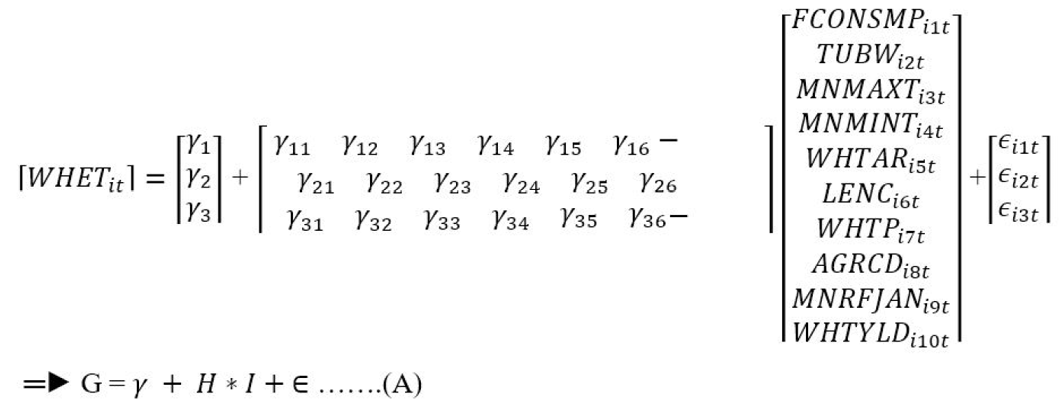
Where dependent variable is the wheat production is meant by G, γ is a group of constants, H is a group of coefficients, the independent variables are indicated by I matrix and ϵ the group of error terms. In matrix I, the consumption of fertilizer for each hector is denoted by FCONSMPi1t. The number of tube-wells used for irrigation purpose is represented by TUBWi2t, MNMAXTi1t and MNMINTi2t are the yearly average of the maximum and minimum temperature in a year respectively, the cultivated area of wheat per hector is defined as WHTARi5t, a proxy used for environmental degradation in logarithm form of energy consumption is denoted by LENCi6t, AGRCRDi8t, Agricultural Credit specified per hector, Price of wheat is denoted by WHTPi7t, WHTYLDi10t is the wheat yield per hector, MNRFJANi9t is yearly average precipitation in January.

The following model is incorporated to measure the impact of self-determining indicators on sugarcane production,

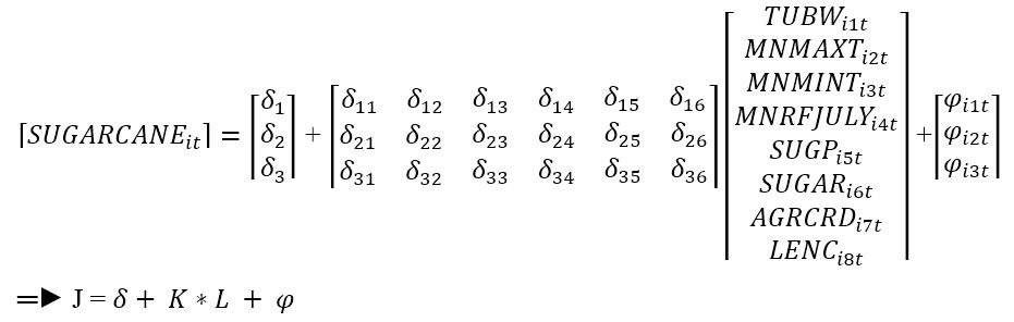
Where the dependent variable is the output of SUGARCANEit, δ is characterized as a constant matrix, K is a matrix of coefficients, independent variables is defined as L matrix and φ is group of error terms. In group L, tube-wells fitted for irrigation is labeled as TUBWi1t. A proxy of environmental degradation in logarithm form of energy consumed is denoted as LENCi8t. MNMAXTi1t and MNMINTi2t are the yearly average of the maximum and minimum temperature in a year, respectively, the yearly average of rainfall in July is denoted by MNRFJULYi4t, AGRCRDi7t, Agricultural credit is given per hector, SUGPi5t, the market price of sugarcane SUGARi6t cultivated area of sugarcane per hector.

The following model is incorporated to capture the impact of the independent variables on land revenue;

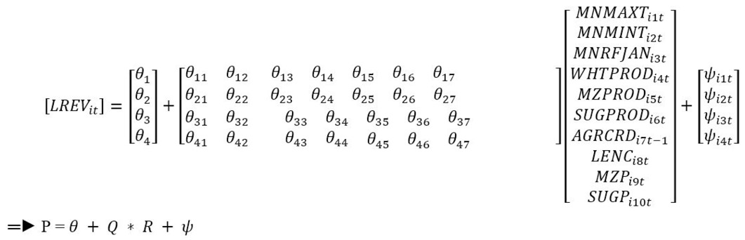
Where P is defined as dependent indicator which is LREVitt, θ is meant by group of constants, Q is a group of coefficients, the independent variables are denoted as R matrix represent and ψ is an error term. In matrix R, MNMAXTi1t and MNMINTi2t are the yearly average of the maximum and minimum temperature in a year, respectively, MNRFJANi3t is the annual mean of rainfall in January, WHTPRODi4t is wheat production level per hector, MZPPRODi5t is maize production level per hector, SUGYLDi6t is sugarcane production level per hector, AGRCRDi7t-1 is lag the value of agricultural credit given per hector, LENCi8t, logarithm form of energy consumption as used for a proxy of environmental degradation, MZPi9t is the market price of maize, SUGPi10t is the market price of sugarcane.

Results and Discussion

Rank analysis result

Table 1, indicates that Punjab leads in wheat production and cultivated area for this crop but at second place in wheat yield and Punjab meet the maximum demand of wheat in the country. Sindh province stands at the second position in wheat production and its cultivated area for wheat but the wheat yield is highest among other provinces. Sindh is self-sufficient in wheat production, which is over and above its domestic needs, and here wheat prices are lower than in other provinces. Khyber Pakhtunkhwa (KPK) province reserved third place for wheat production and cultivated area of wheat, but it has the lowest wheat yield than other provinces. Here the demand for wheat is more than its supply that is why wheat prices are at extreme as associated to other provinces. Khyber Pakhtunkhwa (KPK) and Baluchistan provinces are at third and fourth place respectively in wheat production, cultivated area and inverse of that in wheat yield. Baluchistan is at least place in all respects because of poor infrastructure and insufficient water resources.

Punjab holds the leading position in sugarcane production and cultivated area, whereas Sindh is at third, fourth and second place in sugarcane production, yield and cultivated area respectively, which means Sindh is not utilizing its resources but KPK has significant sugarcane production and exports maximum its production to Afghanistan. Sugarcane prices are less in Punjab as compared to KPK and Sindh, it means sugarcane is more demanded in these two provinces or excess supply of sugarcane exist in Punjab. Punjab is leading in sugarcane production and cultivated area and second place at sugarcane yield. Baluchistan is the least one among other provinces in all respects as Baluchistan is self-sufficient in fruit production and it fulfills the country’s needs and exports it as well.

The land revenue situation in Sindh and Baluchistan prevails at third and fourth place, respectively; it is because of price variation and abundant land existing to tenants at rent. There is an inverse relationship between the supply of land and land rent and due to excess supply of land, which forces the landlord to get lower rent. The Punjab and KPK provinces facedifferent where ownership of land is not too much, typically growers utilize their land for self-use and minimum land is available on rent. Hence, worth of land rent is high in these two provinces than other provinces. Common growers of KPK and Punjab export wheat and sugar to Afghanistan to generate revenue for them, but it leaves the local market in disequilibrium, later on, authorities in Pakistan have to import wheat to fulfill food scarcity in the local market. It indicates that ignoring long-run benefits to secure short-term benefits creates problems for the society.

Table 2 describes the equation for the consumption of fertilizer, tube-wells agricultural credit, and land revenue. The maximum use of fertilizer and agricultural

 

Table 1: Rank analysis of provinces for the production, yield, cultivated area and price of wheat and sugarcane, respectively.

Provence	Production		CROP Yield		Cultivated Area		Respective Price
	Wheat	Sugarcane	Wheat	Sugarcane	Wheat	Sugarcane	Wheat	Sugarcane
Baluchistan	4	4	3	3	4	4	2	4
KPK	3	2	4	1	3	3	1	1
Punjab	1	1	2	2	1	1	3	3
Sindh	2	3	1	4	2	2	4	2

Source: Authors estimation.

 

credit is in Sindh, but the production is not up to that level that was considered, this shows other interests are served through agricultural credits instead of farming. Baluchistan secured the last position in agricultural credit and fertilizer uses on having fewer chances they in this respect. It might surge with the improvement of the cultivated area, while fixing of tube-wells remained at third place for Baluchistan, tube-well is the main source of watering there.

 

Table 2: Rank analysis of provinces for the use of fertilizer, agricultural credit, tube-wells and land revenue.

Province	LREV	FCONSP	AGRCRD	TUBW
Baluchistan	4	4	4	3
KPK	2	3	3	4
Punjab	1	2	2	1
Sindh	3	1	1	2

Source: Authors estimation.

 

Table 3: Environmental statistics of the provinces of Pakistan.

Province	MNMAXT	MNMINT	MNRFJAN	MNRFJULY	LCO2	LENC
Baluchistan	1	4	1	2	4	3
KPK	4	3	3	3	3	2
Punjab	3	2	2	1	1	4
Sindh	2	1	4	4	2	1

Source: Authors estimation.

 

Table 3 indicates the provincial positions of environmental statistics in respect to energy uses and emission of harmful gasses which are responsible for global warming. The average of precipitation in Punjab is high as compared to other provinces whereas the maximum and minimum temperature is at the moderate position whereas Sindh is at second place in this regard. The energy consumption in Punjab is at least position, even then the emission of gasses is at a high degree in Punjab and Sindh but with high energy consumption due to significant industrial setup, it means these two provinces are not considering pollution measures in said areas. KPK is listed third in all climatic variables, Baluchistan has diverse outcomes and validate first in maximum temperature and sensible consequence in average precipitation, emission of CO2 release is insignificant and energy use, due to smallest manufacturing structure accessible in the province. KPK and Sindh are at third and fourth place in rain fall in January and July, respectively. Whereas Baluchistan and Punjab are at first and second place in January rainfall but holding position of inverse of that in July. Baluchistan is not benefitting from rainfall position due to least infrastructure of storing water resources and canal system.

Empirical analysis

Table 4 shows that in all four models, tube-wells (TUBW) are considered; having a direct and significant association with the dependent variable, as well as wheat production has the same results. The first two models contain Fertilizer consumption (FCONSP) where it is positive and significant, it can be seen that the consumption of fertilizer is directly proportional to the production level of crops. The public lacks in provision of agricultural accessories then the private sector steps forward to regulate supply channels and to contribute to the Agro-economy, (Jayne et al., 2003). All four models contain a cultivated area for Wheat (WHTAR) production proves direct and significant for each OLS and FE analysis. In the third and fourth models, the wheat yield is included for which it has a direct and significant association with the dependent variable and for second model the wheat price (WHTP) is positive and insignificant, and Agricultural credit (AGRCRD) is positive and significant.

All four models contain the average of maximum temperature (MNMAXT), where it has direct and significant impact, which indicates a crucial need for the maximum temperature at the final stage for wheat production. The average of minimum temperature (MNMINT) is considered in the first model and found positive and significant here. Beyond the threshold stage, the food value diminishes with rising temperature. The average of precipitation in January (MNRFJAN) surges the production up to a significant level. In the first model, Logarithm form of Energy Consumption (LENC) is comprised where it has as inverse and insignificant relationship, indicating that it has inverse impact but not proves it harmful for the dependent variable, whereas, in second and third models, it has an inverse and significant impact with the dependent variable. This means that with the increase in energy uses, the environment destroys and harmfully upsets wheat production.

Table 5 shows that tube-wells that are taken in the first model only; here it has a direct and significant association with Sugarcane production (SUGPROD) as a dependent indicator. In all four models, agricultural credit, sugarcane cultivated area and its price in second model only are considered, where they are positive and significant. The facility of agricultural credit improves the capability of growers to compensate advanced technology, hybrid seed in the production process. In the last three models, average of the maximum and minimum temperature is jointly considered, MNMAXT has direct and significant relationship with dependent variable, whereas, the average of minimum temperature (MNMINT) has a inverse but insignificant association with the dependent variable.

In all four models average of precipitation in July (MNRFJULY) is included; it proves direct and significant association with the depended variable, which means MNRFJULY is much desirable for sugarcane to reinforce growing procedure at early phase. Second and third models contain a logarithm form of energy consumption (LENC), have a negative and significant association with the dependent indicator, it means, with an increase in energy uses, sugarcane production got adverse impacts. Whereas, the first and the fourth models are negative and insignificant.

Table 6 defines that maize and sugarcane production creating positive and significant over land revenue, where wheat production is positive and significant only second model and insignificant in rest of three models. While sugarcane and wheat prices are considered in second model only where these are positive and insignificant for the dependent variable. It indicates that crop prices frequently fluctuate and yield least inspirations for grower to get more land on rent from the land lord to enhance their income level. The average of maximum temperature (MNMAXT) and minimum temperature (MNMINT) are comprised in the last three models, whereas, MNMAXT showed a positive and insignificant relationship with dependent variable and MNMINT showed a positive and

 

Table 4: Regression analysis of wheat production as dependent variable.

Variables	OLS				FE
	Model-1	Model-2	Model-3	Model-4	Model-1	Model-2	Model-3	Model-4
FCONSP	1.3785	1.889			1.759	1.0496
	(2.732) *	(3.63) *			(1.92) **	(1.68) ***
TUBW	0.0046	0.0026	0.4409	2756.6	0.0056	0.005	0.0038	0.06911
	(4.086) *	(1.77) ***	(7.90) *	(12.05) *	(3.474) *	(2.892) *	(4.14) *	(8.59) *
MNMAXT	30.357	26.138	21.88	33.19	49.629	52.955	19.993	18.55
	(2.48) **	(2.021) **	(1.86) **	(1.70) ***	(2.984) *	(3.365) *	(2.39) *	(2.354) *
MNMINT	25.543				12.205
	(2.419) *				(1.98) **
MNRFJAN			4.4868	3.39			4.4431	3.624
			(2.44) *	(1.96) **			(2.05) *	(1.94) **
WHTP		0.073				0.7142
		-0.443				-0.76
WHTYLD			1.0492	1.004			0.8464	0.781
			(7.162) *	(6.28) *			(5.34) *	(4.26) *
WHTAR	1.53252	1.555	3.1007	1.831	1.4579	1.4375	3.671	1.564
	(17.65) *	(15.79) *	(8.719) *	(18.96) *	(9.044) *	(12.98) *	(7.42) *	(5.89) *
AGRCRD		0.0114				0.027
		(1.87) **				(1.90) **
LENC	-328.12	-1115.83	-1544.51		-716	-1022.9	-1427.07
	(-0.46)	(-2.197) *	(-3.23) *		(-0.586)	(-2.40) *	(-2.09) **
Constant	-1777.2	-1308.1	-3986.82	-1753	-1016.86	-1099.55	-4896.01	-1028
	(-2.07) **	(-2.1) **	(-4.52) *	(-2.15) **	(-0.767)	(-1.29)	(-4.85) *	(-0.749)
Ad.R2	0.994	0.9946	0.996	0.9959	0.99502	0.9952	0.996	0.995
F-Stat	(728.4) *	(280.0) *	(325.6) *	(276.0) *	(650.5) *	(645.2) *	(956.8) *	(726.8) *
Obs.	92	91	92	92	91	91	92	91

Source: Authors estimation. Significance level:*<1 %, **<5 %,***<10%

 

Table 5: Regression analysis of sugarcane production as dependent variable.

VARIABLES	OLS				FE
	Model-1	Model-2	Model-3	Model-4	Model-1	Model-2	Model-3	Model-4
TUBW	0.0042				0.003
	(8.09) *				(5.08) *
MNMAXT	1.784		1.827	1.455	1.94		2.067	2.043
	(1.87) **		(1.97) **	(1.92) **	(1.83) * *		(2.404) *	(2.143) *
MNMINT		2.562	2.204	1.8		0.422	0.118	0.57
		-1.437	-1.53	-0.61		-0.317	-0.044	-0.22
MNRFJULY	0.575	0.403	0.306	0.48	0.39	0.383	0.391	0.379
	(3.546) *	(1.96) **	(1.98) **	(2.75) *	(1.95) * *	(1.90) **	(1.84) **	(2.15) *
SUGP		0.693				0.893
		(2.406) *				(5.308) *
SUGAR	1.21	0.835	0.524	0.944	0.0041	1.0714	0.548	0.595
	(15.27)*	(8.86)*	(3.091)*	(9.18)*	(6.86)*	(12.81)*	(3.26)*	(4.64)*
AGRCRD	0.005	0.002	0.002	0.002	1.1	0.0106	0.022	0.021
	(8.74)*	(3.155)*	(3.67)*	(3.57)*	(10.38)*	(2.13)*	(3.99)*	(3.90)*
LENC	-69.38	-1596.06	-1216.41	-170.1	-26.79	-1494.35	-1230.49	-164.2
	(-1.62)	(-2.743)*	(-2.47)*	(-1.68)	(-0.501)	(-2.55)*	(-2.38)*	(-1.45)
Constant	-149.38	-97.705	-136.84	-241.17	-123.58	-182.53	147.1275	221.2889
	(-3.08)*	(-0 .88)	(-0.91)	(-1.81)**	(-2.52)**	(-2.048)*	-1.0008	-1.63
Ad.R2	0.9731	0.951	0.955	0.952	0.979	0.979	0.972	0.972
F-Stat	(472.13)*	(293.34)*	(243.88)*	(231.57)*	(158.78)*	(149.69)*	(106.95)*	(109.79)*
Obs	92	92	92	92	92	92	92	92

Source: Authors estimation. Significance level:*<1 %, **<5 %,***<10%

 

Table 6: Regression analysis of land revenue as dependent variable.

VARIABLES	OLS				FE
	Model-1	Model-2	Model-3	Model-4	Model-1	Model-2	Model-3	Model-4
WHTPROD	0.090 (0.282)	0.195 (2.06)*	0.108 (0.58)	0.058 (0.531)	0.096 (0.22)	0.257 (2.508) *	-0.145 (-0.66)	-0.096 (-0.57)
MZPROD	1.73 (20.4)*	0.62 (3.16)*	0.733 (2.75)*	0.428 (1.83)*	1.81 (19.6)*	0.565 (2.77)*	0.54 (1.68)*	0.469 (1.79)**
SUGPROD	2.282 (1.96)**	4.518 (2.58)*	6.30 (3.05)*	3.83 (2.20)*	2.49 (1.9)**	3.98 (2.85)*	4.123 (2.72)*	2.62 (1.92)* *
AGRCRD(-1)		0.120 (6.51)*	0.14 (6.87)*	0.133 (7.05)*		0.133 (6.41)*	0.147 (6.45)*	0.148 (6.65)*
MNMAXT		66.53 (1.6)	24.32 (0.55)	16.82 (0.38)	67.28 (1.51)		25.12 (0.75)	56.60 (0.81)
MNMINT		59.80 (1.88)**	123.38 (2.67)*	71.405 (2.160)*		66.46 (2.11)*	74.40 (2.30)*	82.89 (2.44)*
MNRFJAN	-8.063 (-0.95)	-2.143 (-0.24)	-0.136 (-0.15)		-22.94 (-1.9)**	-2.71 (-0.24)	-6.95 (-0.59)
LENC		-1684.4 (-2.41)*	-2167.23 (-2.44)*	-627.72 (-0.37)		-660.21 (-2.485)*	-1994.65 (-2.79)*	-1700.33 (-1.30)
MZP	1.64 (.88)				1.99 (0.91)
SUGP	3.67 (0.70)				3.63 (0.64)
Constant	-5331.55 (-6.09)*	-2522.41 (0.130)*	-4021.99 (-1.51)*	-2647.57 (-1.167)*	-6134.15 (-3.31)*	-843.93 (-0.44)*	-4107.30 (-1.23)	-1649.21 (-0.518)
Ad.R2	0.880	0.877	0.88	0.884	0.870	0.88	0.88	0.961
F-Stat	(71.29)*	(89.24)*	(64.85)*	(66.88)*	(39.69)*	(24.60)*	(22.42)*	(74.56)*
Obs.	87	87	87	87	87	87	87	87

Source: Authors estimation. Significance level:*<1 %, **<5 %,***<10%

 

significant relationship with the dependent variable. In all models, average of precipitation in January (MNRFJAN) is comprised, whereas, it is a negative but insignificant. LENC is negative and significant for second and third models but insignificant for first and fourth models.

Conclusions and Recommendations

Pakistan possesses world major canal structure but failed to construct water reservoir due to political clashes and facing worst energy disasters. Pakistan’s capability to rescue climatic disasters is uncertain, since it has the least technical infrastructure, skills and resources are ordinary one, mainly through out rainy season. Cumulative pollution is one the problem that Pakistan is facing mainly in industrial zones and cities. According to law industrial sector liable to emission of gasses into environment but ignorance both at industrial and legal sides creating environmental problems which are being worst day by day in the Pakistan economy. The maximum and minimum temperatures are positive and significant for wheat land revenue but negative and significant for sugarcane. The agricultural accessories like fertilizer, tube-well, agricultural credit etc., creating positive and significant impacts on crop production and land revenue. For the production level, cultivated area and crop yield province Punjab and are Sindh are in leading position, whereas KPK and Baluchistan are taking highest position in pricing of respective crops. The political unrest in the society is proving hard for decision making at Government level to save the society. Pakistan is one of those countries that are sensitive to climate change. The present study is the subject of an examination of whether climate change is affecting the production of wheat, sugarcane and land revenue, which are the source of farmer’s income. A panel data approach is used to analyze the data for each province of Pakistan. Results are presented using rank and regression analysis. The rank analysis was based on fertilizer use, number of tube-wells, and respective prices. It is found that the Punjab province is at the top in the majority of elements and Baluchistan holds the least position in this regard. In regression analysis, the climatic index was found negative and significant, whereas agricultural accessories are positive and significant with the dependent variables. This study recommends to rationalize the use of certain factors of production, such as fertilizer and energy consumption that negatively affect the environment. It suggests the use of other resources, such as tube-wells and provision of credit to farmers that positively impact the major crops and land revenue in Pakistan.

Novelty Statement

This study provides valuable information about the impact of environmental degradation and agricultural accessories on crops and land revenue in Pakistan. It suggests recommendations for reducing environmental degradation and promoting agricultural accessories to ensure sustainable income for farmers.

Author’s Contribution

Naveed Wahid Awan: Idea, write-up, data collection and analysis.

Asif Ali Abro: Helped in data collection, estimation and correction of grammatical errors.

Ahmed Raza ul Mustafa: Helped in estimation and proof reading of manuscript.

Conflict of interest

The authors have declared no conflict of interest.

References

Abd-Halid, A., Q. Meng, L. Zhao and F. Wang. 2009. Field study on indoor thermal environment in an atrium in tropical climates. Building and Envi., 44(2): 431-436. https://doi.org/10.1016/j.buildenv.2008.02.011

Abro, A.A. and I.A. Panhwar. 2020. Impact of various factors on crop diversification towards high value crops in Pakistan: An empirical analysis by using THI. Sarhad J. Agric.,36(4): 1254-1265. https://doi.org/10.17582/journal.sja/2020/36.4.1254.1265

Abro, A.A., N.W. Awan and M.A.P. Panhwar. 2020. Effects of untreated sewage on marine environment-a case study of Karachi. Int. J. Agric. Biol. Sci., Sep and Oct 2020, 147-157.

Blanc, E. and W. Schlenker. 2017. The use of panel models in assessments of climate impacts on agriculture. Rev. Environ. Econ. Policy, 11(2): 258–279. https://doi.org/10.1093/reep/rex016

Gbetibouo, R.M. Hassan and C. Ringler. 2010. Modelling farmers’ adaptation strategies for climate change and variability: The case of the Limpopo Basin, South Africa. Agrekon, 49(2): 217-234. https://doi.org/10.1080/03031853.2010.491294

GoP. Economic Survey of Pakistan. 2018-19. Economic Advisor’s Wing, Finance Division, Islamabad. http://www.finance.gov.pk/survey_1819.html

Jan, T.M., E.M. Lenaerts, R. Michiel, V.D. Broeke, R.M. Stefan, R.M. Ligtenberg, M. Horwath and E. Isaksson. 2013. Recent snowfall anomalies in Dronning Maud Land, East Antarctica, in a historical and future climate perspective. Geophys. Res. Lett., 40(11): 2684-2688. https://doi.org/10.1002/grl.50559

Jayne, T.S., T. Yamano, M.T. Weber, D. Tschirley, R. Benfica, A. Chapoto and B. Zulu. 2003. Smallholder income and land distribution in Africa: implications for poverty reduction strategies. Food Policy, 28(3): 253-275. https://doi.org/10.1016/S0306-9192(03)00046-0

Kumar, K., K.R. Kumar, R.G. Ashrit, N.R. Deshpande and J.W. Hansen. 2004. Climate impacts on Indian agriculture. Int. J. Climatol. J. R. Meteorol. Soc., 24(11): 1375-1393. https://doi.org/10.1002/joc.1081

Kurukulasuriya, P. and R. Mendelsohn. 2008. Crop switching as a strategy for adapting to climate change. Afr. J. Agric. Resour. Econ., 2(311-2016-5522): 105-126. https://ageconsearch.umn.edu/record/56970/

Linwood, P., P. King, M. Craig, D.G. Webster, R. Vaughn and P.N. Adams. 2011. Estimating the potential economic impacts of climate change on Southern California, beaches. Clim. Change, 109(1): 277-298. https://doi.org/10.1007/s10584-011-0309-0

Louise, A., K. Hope, W.J. Alonso, V.D. Thiem, D.G. Canh, D.A. Marguerite, A. Xenopoulos, D.M. Lodge, J. Alcamo, M. Marker, K. Schulze and D.V. Vuuren. 2005. Scenarios of freshwater fish extinctions from climate change and water withdrawal. Glob. Change Biol., 11(10): 1557-1564. https://doi.org/10.1111/j.1365-2486.2005.001008.x

Marguerite, A., D. Xenopoulos, M. Lodge, J. Alcamo, M. Marker, K. Schulze and D.P.V. Vuuren. 2005. Scenarios of freshwater fish extinctions from climate change and water withdrawal. Glob. Change Biol., 11(10): 1557-1564. https://doi.org/10.1111/j.1365-2486.2005.001008.x

Martin, P., C. Rosenzweig, A.G. Fischer and M. Livermorea. 1999. Climate change and world food security: A new assessment. Glob. Environ. Change, 9: 51-S67. https://doi.org/10.1016/S0959-3780(99)00018-7

Michael, A., B.X. Zeng, V. Misra and A. Beljaars. 2008. Integration of a prognostic sea surface skin temperature scheme into weather and climate models. J. Geophys. Res. Atmospheres, 113(D21). https://doi.org/10.1029/2008JD010607

Molua, E. and Lambi, 2007. The economic impact of climate change on agriculture in Cameroon. World Bank Policy Research Working Paper, (4364).

Nellemann, C., M. Devette, M. Manders, T. Eickhout, B. Srihas, B. Prins and A.G. Kaltenborn. 2009. The environmental food crisis: The environment’s role in averting future food crises: A UNEP rapid respons assessment.

Polsky, C., 2004. Putting space and time in Ricardian climate change impact studies: Agriculture in the US Great Plains, 1969–1992. Ann. Assoc. Am. Geogr., 94(3): 549-564. https://doi.org/10.1111/j.1467-8306.2004.00413.x

Qin, D.D.Y., S.U. Jilan, R.E.N. Jiawen, W. Shaowu, W.U. Rongsheng, Y. Xiuqun, W. Sumin, L. Shiyin, D. Guangrong, L. Qi, H. Zhenguo, D. Bilan and L. Yong. 2005. Assessment of Climate and Environment Changes in China (I): Climate and environment changes in China and their projection. Adv. Clim. Change Res., 1(002).

Reinsborough, M.J., 2003. A Ricardian model of climate change in Canada. Can. J. Econ., 36(1): 21-40. https://doi.org/10.1111/1540-5982.00002

Revadekar, J., Y.K. Tiwari and K.R. Kumar. 2012. Impact of climate variability on NDVI over the Indian region during 1981–2010. Int. J. Remote Sens., 33(22): 7132-7150. https://doi.org/10.1080/01431161.2012.697642

Richard, M., A.C. Chang, B.A. McCarl and J.M. Callaway. 1992. The role of agriculture in climate change: A preliminary evaluation of emission control strategies. Econ. Issues Glob. Clim. Change: Agric. For. Natl. Resour., pp. 273-287.

Robert, M., W.D. Nordhaus and D. Shaw. 1994. The impact of global warming on agriculture: A Ricardian analysis. Am. Econ. Rev., 753-771. https://www.jstor.org/stable/2118029?seq=1

Robert, M., 2000. Efficient adaptation to climate change. Clim. Change, 45(3-4): 583-600. https://link.springer.com/article/10.1023/A:1005507810350

Sajjad, S.H., S.A. Shirazi, M.A. Khan and A. Raza. 2009. Urbanization effects on temperature trends of Lahore during 1950-2007. Int. J. Clim. Change Strat. Manage., 1(3): 274-281. https://doi.org/10.1108/17568690910977483

Smith, P. and J.E. Olesen. 2010. Synergies between the mitigation of, and adaptation to, climate change in agriculture. J. Agric. Sci., 148(5): 543-552. https://doi.org/10.1017/S0021859610000341

Stephanie, M.D., N.L. Bindoff and S.R. Rintoul. 2009. Impacts of climate change on the subduction of mode and intermediate water masses in the Southern Ocean. J. Clim., 22(12): 3289-3302. https://doi.org/10.1175/2008JCLI2653.1

Suman, J., 2007. An empirical economic assessment of impacts of climate change on agriculture in Zambia. The World Bank.

Sung-No, N.S., R. Mendelsohn and M. Munasinghe. 2005. Climate change and agriculture in Sri Lanka: a Ricardian valuation. Environ. Dev. Econ., 10(5): 581-596. https://doi.org/10.1017/S1355770X05002044

Timmer, C.P., 2010. The changing role of rice in Asia’s food security. https://www.think-asia.org/handle/11540/1396

Yair, M., D. Larson and R. Butzer. 2004. Agricultural dynamics in Thailand, Indonesia and the Philippines. Aust. J. Agric. Resour. Econ., 48(1): 95-126. https://doi.org/10.1111/j.1467-8489.2004.00231.x