
Precise Yield Estimation through Improvised CASA Model by Development of Soil and Atmospheric Constants (Sᵮ) and (Aþ)


Research Article
Precise Yield Estimation through Improvised CASA Model by Development of Soil and Atmospheric Constants (Sᵮ) and (Aþ)
Rao Mansor Ali Khan* and Syed Amer Mahmood
Department of Space Science, University of the Punjab, Lahore, Pakistan.
Abstract | Net Primary Production (NPP) is an indicator that is widely used to determine the supply of food and wood. NPP incorporates almost all factors that participate in the growth and development of a particular crop. These factors include various heat fluxes (e.g., ground, sensible and latent heat flux), a variety of radiations (e.g., extraterrestrial, shortwave, longwave, and net radiations), and the photosynthesis index. In this research, the net radiations were estimated as 27,428 Wm−2 throughout the wheat growth period (WGP), including (118.3 Wm−2) as shortwave and (34.63 Wm−2) as longwave radiation. Latent, soil and latent heat fluxes were estimated as 3324 Wm−2, 16,549 Wm−2, and 7554 Wm−2, respectively. Water stress during the complete WGP ranged between 0.5838 and 0.1218 from the start to the end of the cultivation period. The biomass creation was estimated as6.09–1.03 g/m2 /day, which was higher at the start of WGP than declined at the end. Finally, the estimated yield was very different as compared to the actual yield. The yield estimated through the CASA(Carnegie–Ames–Stanford approach) model was uniform for the complete study site; however, the actual yield was about 74% less than CASA generated yield in various plots. This issue was further investigated and found that the CASA model lacks various aspects. These aspects include soil suitability parameters, including pH, Organic matter, CaCO3, texture, and Electric Conductivity. The largest gap inthe CASA model, which affected the overall productivity of wheat, was the smog/haze factor which was not incorporated. The environmental factors include Black Carbon (BC), Carbon monoxide (CO), Nitrogen dioxide (NO2), Ozone (O3), and Sulphur dioxide (SO2). To cater to these issues, two indicators were developed to incorporate the smog and soil-related issues. These indicators are named Soil Factor (Sᵮ) and Atmospheric Factor (Aþ). If the soil is “Not Suitable,” the values of Sᵮ is 0.147, for less suitable soil Sᵮ is 0.21, for moderately suitable soil, Sᵮ is 0.61, and for highly suitable soil, Sᵮ is 0.95. By substituting these values of Sᵮ, the overall results approach to actual yield by 96%. The other factor Aþ is based on incorporating the situation of Atmospheric conditions faced by the wheat crop canopy, whichinclude Black Carbon (BC), Carbon monoxide (CO), Nitrogen dioxide (NO2), Ozone (O3), and Sulphur dioxide (SO2) parameters. If the overall air quality is conducive, the value of Aþ is near 1. The results obtained through the improved CASA model by the addition of Sᵮ and Aþ provided a very accurate yield that was near to actual estimates.This study is important to obtain precise estimates of cereal crops incorporating physio-climatic factor that leads toward precision agriculture.
Received | September 15, 2022; Accepted | October 04, 2022; Published | December 29, 2022
*Correspondence | Rao Mansor Ali Khan, Department of Space Science, University of the Punjab, Lahore, Pakistan; Email: raomansor@gmail.com
Citation | Khan, R.M.A. and S.A. Mahmood. 2022. Precise yield estimation through improvised CASA model by development of soil and atmospheric constants (Sᵮ) and (Aþ). Sarhad Journal of Agriculture, 38(5): 355-371.
DOI | https://dx.doi.org/10.17582/journal.sja/2022/38.5.355.371
Keywords | Net primary production (NPP), Respiration and CASA model, Biomass estimation and water stress,Wheat cultivation period, Net radiation and photosynthesis
Copyright: 2022 by the authors. Licensee ResearchersLinks Ltd, England, UK.
This article is an open access article distributed under the terms and conditions of the Creative Commons Attribution (CC BY) license (https://creativecommons.org/licenses/by/4.0/).
Introduction
Wheat (Triticumaestivum) provides about 20% of the entire nutrient and protein needs of 4.5 billion people, with a total harvesting area of 215.9 Mha (Luo et al., 2022). Due to the tremendous rise of the world’s population, which is projected to reach 9 billion by 2050, wheat output must double to meet demand (Nelson et al., 2010). 37% of worldwide wheat harvesting areas have seen output stagnation in recent years, threatening the capability of agricultural output to fulfill increasing worldwide consumption (Luo et al., 2022).
The scarce production of wheat is inadequate to fulfillthe needs of society around the globe. Climate changes and population increases in wheat-producing countries haveput huge pressure on increasing wheat yield (Reynolds et al., 2010; Xiao et al., 2005). Modern agricultural practices must be applied to ensure sustainable production of wheat yield. In short time, the accurate estimation of NPP of the wheat crop hasbecome quite difficult for economists and agronomists. NPP is a renowned indicator to estimate the overall production for determining the shortfall or surplus to take in time decisions for importing or exporting of wheat grains. Multiple factors affect the NPP which include microbial characteristics of soil, climate, anthropogenic activities and topography of soil (Field et al., 1995; Zhu et al., 2017).
The key agricultural processes are respiration and photosynthesis,whichplay a key role in plant production under sunlight (Guoshui et al., 2011; Lima et al., 2012). A detailed description of the productivity of the soil can be obtained by analyzing the effect of sunlight on the growth of the plant in its sequential stages (Pachavo and Murwira, 2014; Scurlock et al., 2002).
Various biomes can be distinguished by analyzing terrestrial NPP. Carbon emissions and sequestrations can be analyzed through significant knowledge of NPP (Maselli et al., 2013; Wang et al., 2013). Analysis of NPP is used to indicate the consumption of carbon dioxide by plants which is a necessary component required for plant growth (Canadell et al., 2000). The ecological disturbance on regional and global scales can be analyzed by estimating NPP (Piao et al., 2006). Multiple climatic factors, including pressure, relative humidity, actual vapor pressure, various solar fluxes (i.e., shortwave radiations, longwave radiations, net radiations, ground heat flux, sensible heat flux, and latent heat flux), and temperature were used by various researcher to estimate NPP (Cramer et al., 1999; Eisfelder et al., 2014; Lehuger et al., 2010) however, it cannot be accurately computed on a large scale, but accuracy up to 74% has been achieved by various researchers at local scales (Lauenroth et al., 2006). NPP was primarily estimated through the Miami model by correlating several productivity levels under the influence of average precipitation and temperature without analyzing other climatic factors (Lin et al., 2013). A variety of methods have been developed using satellite data by the evolution of remote sensing technology, and these techniques can be used to estimate the NPP of the terrestrial ecosystem (Lin, 2009). Carnegie-Ames-Stanford Approach (CASA) model is based on satellite data that incorporates Light Use Efficiency (LUE) to correlate the climatic variables for estimation of NPP (Lieth, 1975). Many researchers have utilized the CASA model in Africa, Eurasia, South America, Australia, and North America (Potter, 2014). A study on global climatic changes sbeen conducted in China utilizing the CASA model, which illustrated its efficacy in determining the progression of agro-industry (Potter et al., 1993b). However, the CASA model has some limitations;for instance, the maximum value of LUE is fixed, that is, 0.389 GC/MJ for all kinds of vegetation (Liang et al., 2015). The CASA model has another limitation, that is, the enumeration of soil capacity, which is related to several other parameters of soil, including soil type, field moisture, and water holding capacity of the soil. The soil parameters may not be estimated accurately to great highextents because of their high spatial diversity.
CASA model is NPP (Net Primary Productivity) derived model, which provides a difference between the amount of organic matter generated by photosynthesis and the amount of organic matter lost to autotrophic respiration. Various factors including climate, soil, nutrient, and CO2 levels play a vital role of existing carbon for the terrestrial ecosystems. The term climatic potential productivity is used to describe the biological or agricultural yield per unit area of land that may be obtained under ideal conditions. This is based on the assumption that vegetation can make full use of climate resources like light, heat, and water. As one of the most important metrics for assessing ecosystem health, NPP is a valuable tool for studying the regional and global carbon cycle through modelling studies. Therefore, it is crucial to have a firm grasp of NPP estimations if we are to accurately predict future carbon budgets in the face of climate change.
Among several models of NPP, three models are considered important in general, which include the process model, the LUE model, and the climatic model (Hicke et al., 2002). The relationship betweenclimatic parameters and NPP is estimated utilizing the climatic model. This model has the limitation that actual and estimated values of NPP consist of large variations; thus, the actual vegetation type may not be considered in this model (Tang et al., 2014).
The process model considers the physiological and ecological parameters, while several soil parameters are phonological, which include photosynthesis, dry matter partition, and respiration (Piao et al., 2005). The phonological parameters under certain environmental conditions cannot be estimated accurately, and nahigh value of uncertainty exists between the estimated and validated NPP (Liu et al., 2012).
The LUE model is quite handy, and isextensively used due to its mechanism. It can be easily combined with remote sensing data. The utilization of solar energy by plants is illustrated by the LUE model considering the energy constant (Deyong et al., 2008). The energy utilized in net production is distributed among all organs of plants which is further transported to the environment. The model comprises the physiological and climatic parameters of vegetation, thus estimatingthe NPP more accurately.
This research is based on a step-by-step hierarchy to estimate biomass utilizing the local environmental factors, including temperature, pressure, humidity, actual vapor pressure, and light use efficiency (Zhu et al., 2021). These factors are handy for computing the various wheat crop growth parameters, including net radiations, ground heat flux, sensible heat flux, water stress, and overall productivity. CASA model provides wage estimates of productivity; therefore, an effort has been made to precisely compute the production with precision by incorporating the soil suitability indicator (ħα) (Raza and Mahmood, 2018); however, there remain many limitations that need to be addressed. These gaps have been taken into account by considering additional parameters essential for wheat crop growth. Therefore, the modified CASA model presented promising results in resemblance with the actual ground-generated yield.
This research is based on various parameters which constitutea process that integrates to provide the generation of biomass on a daily basis throughout the wheat growth period. Climatic data collected through real-time field observations as recorded by Meteorological stations assisted inr computingof various fluxes, e.g., soil heat flux, net radiation flux, latent heat flux, and sensible heat flux that affect the overall productivity. LUE intake by the wheat crop assisted inin analyzing analyzing respiration and photosynthesis (Corey et al., 1997). Change in light use can be determined against each growth stage of the wheat crop that describes various productivity levels in its sequential stages because NDVI varies with variations in LUE. The NDVI values assisted estimating in estimating thebiomass of each day that was later compared with the actual yield as reported by a local farmer. A lack was observed in an overall mathematical model of the Caraneigh Ames Stanford Approach for not incorporating the effect of atmospheric pollutants that lead to the overall estimates of yield beyond the limit (Potter, 1997). An effort was made for precision agriculture by highlighting the loopholes in the CASA model byintroducing the yield precision indicators, e.g., we introduced two factors, Soil Factor (Sᵮ) and Atmospheric Factor (Aþ), and found that the results are 99% near to the actual yield.
Materials and Methods
Investigation site
The study area is located in Pakistan’s Punjab province. This province is Pakistan’s second largest in terms of size and population, accounting for around 56% of the country’s total population (Uauy et al., 2006a). Punjab is regarded as Pakistan’s breadbasket, with 12.4 million hectares of arable land (Uauy et al., 2006b). Wheat was planted on 6.98 million hectares during the Rabi season of 2014-15 (Dempewolf et al., 2014). Punjab is divided into three major agro-ecological zones: I Potwar plateau, which contains 10% of the province’s rain-fed agricultural land; and (ii) Punjab plateau, which contains 10% of the province’s rain-fed agricultural land (Crop Reporting Service, Punjab, 2015), (ii) the semi-arid and dry deserts of central and southern Punjab, which produce less agricultural; (iii) the Indus basin region, which has the highest irrigated crop farming area. Punjab produces wheat and other staple foods that contribute greatly to the state’s economic prosperity (Rabbi et al., 2021). Agriculture provides employment for around 66% of Pakistan’s rural population. The study region, which includes Vehari, MianChannu, Burewala, and Chichawatni, is regarded as one of the greatest wheat producers. Geographically, the examination site is located between 72oE and 73oE longitude and 29.50o N to 30.50o N latitude and is surrounded by extremely fertile soil. The average elevation of investigation site is 145 m. As illustrated in Figure 1, the study region is a subset of the Landsat patch with 150/39 path/row.
The flow of the methodology
The methodology opted in this study to evaluate the total wheat production with local environmental parameters is given in detail in the flow provided in Figure 2.
CASA model
The NPP in the study area is estimated accurately using the CASA model. The CASA model has been developed on the basis of LUE, which is commonly used to estimate the productivity of vegetation at a global scale (Brogaard et al., 2005; Propastin and Kappas, 2009; Rahman As-syakur et al., 2010; Wang et al., 2009). Estimation of LUE is a significant parameter for mapping of NPP, which spatially estimates several parameters of vegetation, e.g., the health of vegetation and water stress, etc. (Li et al., 2012). The LUE illustrates spatial heterogeneity at different levels because of the composition of species and physiological characteristics of vegetation. The LUE is the indispensable parameter of the plant. Multiple factors, including leaf area, chlorophyll content, and growth stages of the plant, influence the LUE at the plant scale. However, canopy structure, leaf inclination angle, LAI, and solar light angle affect LUE at the canopy scale. The utilization of remotely sensed data in LUE identifies the dissimilarity in vegetation at a regional scale by analyzing spatial variability. LUE can be computed through various methods, including the productivity model, Eddy covariance technology model, quantum efficiency reckoning method, and inversion method (Li et al., 2012). The differences in LUE can be computed using site-based measurement and photochemical reflectance index. A positive relationship is determined between Absorbed Photosynthetic Active Radiation (APAR) and NPP. NDVI is used as an input to compute APAR (Clevers et al., 1989). The fraction of light absorption by plants can be computed using the CASA model, which incorporates NDVI. NDVI is linearly related to Photosynthetic Active Radiation (PAR) which is intercepted by the spectral index of the crop canopy (Gitelson, 2018).
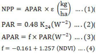
PAR is a fraction of solar radiation having a wavelength between 0.4–0.7 µm, which is available during actual sunshine hours (Escobedo et al., 2011). NPP is computed in the CASA model as a product of LUE and APAR, as illustrated in Equation 1:
The appropriate values of PAR range from 40 to 50 percent to represent the average condition (Moran et al., 2009). (Equation 2)
Where; K24 represents the incident radiation on the wheat crop canopy. The Ratio of PAR and APAR presenteda fraction of available to absorbed radiations for photosynthesis (Ahl et al., 2004; Bird and O’Connell, 2006; Conrad et al., 2010; Runyon et al., 1994) and mentioned below in Equation 3.
The NDVI values are used to estimate fraction f according to (Field et al., 1995) in Equation 4.
Sentinel-2 satellite images are listed in Table 1 to compute Spatio-temporal variations in NDVI throughout the wheat growing season.
Table 1: Sentinel-2 image acquisition dates.
|
S. No. |
Image acquisition dates |
|
1 |
17 November 2019 |
|
2 |
2 December 2019 |
|
3 |
26 January 2020 |
|
4 |
31 January 2020 |
|
5 |
15 February 2020 |
|
6 |
25 February 2020 |
|
7 |
16 March 2020 |
|
8 |
21 March 2020 |
|
9 |
5 April 2020 |
|
10 |
20 April 2020 |
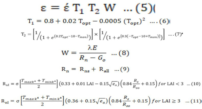
Depending upon the physiological characteristics of plants, the value of LUE varies for various crops (Monteith, 1972). The impact of water stress on LUE was analyzed by (Asrar et al., 1985). Moisture conditions and temperature influence the results, while in ideal conditions, the results are maximal. The LUE for wheat crops was calculated (Khabba et al., 2020) as illustrated in Equation 5.
The maximum conversion factor is determined by έ to compute biomass above the surface of the Earth under optimum environmental conditions, and a value of 2.5 g·MJ−1 is fixed for the wheat crop (Bastiaanssen and Ali, 2003).
T1 and T2 are heat variables, while W indicates water stress on the crop as it grows. LUE may not be greater than έ (Bastiaanssen et al., 1997). T1 shows that LUE reduces with deviations in actual crop temperature as compared to the optimal temperature required for wheat crop growth, whereas T2 shows that LUE decreases with deviations in actual crop temperature compared to the optimal temperature required for wheat crop growth. T1 and T2 were calculated (Bastiaanssen and Ali, 2003; Bradford et al., 2005; Potter et al., 1993a) using Equation 6 and 7.
Top is the mean air temperature for the month with the highest LAI for a certain crop (for example, the highest LAI for wheat crops was recorded in February), and Tumon represents the mean monthly air temperature for the complete crop growth cycle (Equation 8).
Net radiation (Rn)
Rn is the key determinant of the balance of E’ ‘Earth’s energy which determines the Ratio of outgoing and incoming radiations (Wu et al., 2017). The evapotranspiration is estimated accurately, but the closure effects of energy balance affect its accuracy. Thus Rn is estimated accurately to investigate agroclimatic conditions. All chemical and physical processes are regulated by solar radiation present in the atmosphere. Various parameters, including the surface temperature of the leaf, air temperature, dew point, sunshine hours, albedo, sky radiations, pressure, and vapor pressure, are used to compute Rn at local and regional scales.
Rnl is four times the temperature of the Earth’s surface, according to Stephen Boltzman’s law.
Rn is the balance between Rns and Rnl, which is calculated as Equation 9.
In accordance with Stephen Boltzman’s law [40], Rnl is four times the Earth’s surface temperature Equation 10 and 11.
Where; Tmaxk and Tmink are daily maximum and minimum temperatures in Kelvin, ea is actual vapor pressure in KPa, Rs and Rs are incoming and actual/clear sky solar radiation (Wm2), and σ is the Stephen Boltzman constant (= 4.903 × 10⁻⁹ M J K-4 m-2 day-1). Mean temperature values throughout the WGP were obtained from Local Metrological Offices (LMOs).
Extraterrestrial radiation is the flux computed at the outermost layer of the atmosphere denoted as Ra (Adnan et al., 2012). It changes throughout the year due to changes in the inclination angle of the sun (Allen et al., 1998). The fraction of extraterrestrial radiations that strikes the surface of Earth by interaction with atmospheric gases is called actual incoming solar radiation. The atmospheric factors, including haze, cloud, fog, etc., affect the dispersion of sunlight and can be computed according to various types of researchpieces of research (Adnan et al., 2012; Allen et al., 1998; Angstrom, 1924; Beard and Hollen, 1970; Deceased and Beckman, 1982; Revfeim, 1997; Wu et al., 2017).
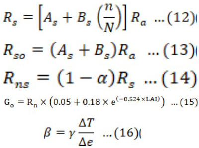
In Equation 12, As and Bs are 0.25 and 0.50, respectively, which are constants (Allen et al., 1998). Where n and N are the actual and maximum sunshine hours, respectively. The variations in n and N for the complete WGP werecollected from LMOs. Extraterrestrial radiations were computed by incorporating month, day, and latitude using the website http://www.engr.scu.edu/~emaurer/tools/calc_solar_cgi.pl. Clear sky radiations are about 75% of extraterrestrial radiations, which determine that 25% of radiations have been scattered, absorbed, or reflected by atmospheric gases. Rso can be calculated using the Angstrom’s formula (Adnan et al., 2012); and (Angstrom, 1924) as below in Equation 13.
Net shortwave radiations were computed using incoming solar radiations and albedo according to (Wu et al., 2017; Angstrom, 1924).
Runs arecomputed in watt/m2 according to Equation 14, and the crop albedo of the wheat crop was substituted as 0.19, particular for the wheat crop (Giambelluca et al., 1997; Oguntunde et al., 2007; Tsai et al., 2007).
Soil heat flux calculation (Go)
The characteristics of soil determine the capacity of soil for conduction of heat due to temperature gradient is represented by soil heat flux (Go) (Sauer and Horton, 2015). Temperature is a key factor that determines all biochemical processes of soil required for essential plant growth. Although Go has the lowest contribution in the energy balance equation, its exclusion may lead to considerable errors. However, excluding it may result in significant errors. Go can be computed as Equation 15.
Where; Rn represents net radiation and LAI, which fluctuates with crop growth. LAI estimation is critical because Go is heavily reliant on the density of leaves through which heat can penetrate to raise soil temperature. We collected LAIvalues for the wheat crop in various growth stages from 31 field observations usingthe instrument LAI 2200; these are mentioned in Figure 3.
Latent (λE) and sensible heat flux (H)
Energy distribution in different organs of a plant without changing their state is termed sensible heat flux (Jones and Rotenberg, 2001). Determination of sensible heat and latent heat flux is important; however, it is a difficult process. Whereas the evaporation by vegetation is computed using the energy balance equation while the sensible heat flux is computed by Bowen ratio (β), which can be computed utilizing variations in temperature and vapor pressure for canopy-environment interface as Equation 16.
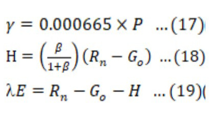
Where γ represents the psychometric constant that is 0.000665 times the atmospheric pressure P (Zotarelli et al., 2014). ∆T and ∆e are temperature and actual vapor pressure gradients, respectively. The expression for γ is Equation 17.
Where; P represents the daily atmospheric pressure in Kpa. ∆T, ∆e, and P were obtained from LMOs and averaged. The Bowen ratio was used to calculate sensible heat (Tanner, 1960) (Equation 18).
The assessment of crop canopy resistance is connected to latent heat flux, which is difficult to quantify since canopy resistance is based on complicated (sometimes non-linear) interactions of plants with atmospheric factors (Monteith and Unsworth, 2013). To avoid using the canopy resistance technique, the residual of the energy balance equation (Tanner, 1960; An et al., 2017; Bowen, 1926; Dicken et al., 2013; Jansen et al., 2011; Mengistu and Savage, 2010; Sauer and Horton, 2015; Venegas et al., 2013) was utilized to calculate the latent heat fluxas (Equation 19).
The spatial information can be extracted using remotely sensed data to simulate carbon dynamics on a global scale (Wulder et al., 2004). Ecosystem models developed using remote sensing datasets are utilized to monitor carbon assimilation globally.
Supervised classification
Land Use Land Cover (LULC) supervised classification on Sentinel-2 satellite multispectral imagery was utilized to estimate the area under wheat cultivation (Phiri et al., 2019), and the Normalized Difference Water Index (NDWI) was applied to get a classified map accurately.
Results and Discussion
Estimation of solar radiation received by wheat crop canopythroughout the WGP
Various solar fluxes, including Rn, Rns, Rnl, Ra, and Rso, were computed, and the results are mapped in Figure 4.
Ra determines the extraterrestrial radiations received at the top of the atmosphere before entering the E’ ‘Earth’s atmosphere; however, the incoming radiations Rso reduces at a rate of 25%, and the rest of 75% is received at the surface of the earth. Ra was recorded as 245.25 w/m2 on 15 November 2019, which increased to 462.2 on 20 April 2020 due to variations in solar angle. Ra, Rs, and Rs for the complete wheat cultivation period were recorded as 50845 w/m2 as Ra, 38133 w/m2 as Rso, whichwas 75% of Ra, and 27753 w/m2 as actual incoming radiation after interaction with the atmosphere. The net radiation Rn wascomputed as 25055 w/m2 with the integrated flux of short wave and long wave radiation that was 19480 w/m2 and 3423 w/m2, respectively. A difference of 2152 w/m2 was observed between net radiations and actual incoming radiations, which were absorbed by the surface of the Earth in the form of heat conduction as ground heat flux Go.
The variations of (n/N) determine the Ratio of actual daylight hours in comparison to total sunshine hours available on a particular day. The estimates determine that 1748 hours were available throughout the WGP while 1012 hours could be received actually due to off and on cloud activity. The Ratio (n/N) is mapped in Figure 5, where the peaks and dips are observed varying between (0-1). The value 1 determines a completely sunny day and 0 indicates a completely cloudy day with 0 sunshine hours.
Estimation of Go throughout WGP
Go was computed by incorporating Rn and LAI and mapped the outcomes in Figure 6. Go is observed to decreasegradually where the highest value of Go was observed as 41.26 w/m2 on 30 November 19, declined to 5.13 w/m2 on 29 January 2020.
The main reason forthe decline in Go is an increase in leave density which was less atthe beginning of the cultivation period that increased with the passage of time. Go is reciprocal of the LAI curve. As LAI increases, Go decreases because high leaf density prohibits the radiation from reaching from reaching earth’s surface.
Estimation of λE and H
The variations in λE and H are mapped in Figure 7 by incorporating Go, Rn, ∆E, P, and T. The estimates show that 21708 w/m2 was absorbed by the wheat crop canopy as a sensible heat flux.
Estimation of W
The water stress was estimated within a range from (0-1) where 1 indicates flooding and 0 represents the oven dry soil (Raich et al., 1991). The water stress was estimated by incorporating Rn, Go, and H, which fluctuated between 0.64 to 0.13. The results in Figure 8 express that there was a surplus of water atthe beginning of cultivation period, and the stress of water was observed in the end near harvesting.
Assessment of LUE
The LUE was estimated for the complete WGP by substituting the value of έ = 2.5 in Equation 5 and mappingthe results in the Figure 9. The wheat crop used more heat in the start of wheat crop growth due to the emergence of new leaves, tillers, and stems and required less heat in the ripening period because of the conversion of milky dough to hard grain.
Assessment of biomass/ NPP
The input parameters, including PAR, APAR, and f are computed to analyze the biomass. The variations in NDVI observed on daily basis are substituted in the Equation 4 in order to calculate the value of f, which varies from 0 to 1. The value of f determines PAR which is utilized as APAR by the wheat canopy for photosynthesis. If the value of f is 0, it indicates the absence of APAR, while the value f=1 shows the equivalence of APAR to PAR. APAR and NDVI are directly related to each other;a decrease in one parameter leads to a drop in the other. Variations in f throughout the WGP areshown in Figure 10.
The biomass was estimated by substituting the Ɛ and APAR in Equation 1 and plotted the results in Figure 10. Biomass was generated for each day of the cultivation period. The results show that NDVI is in direct relation with biomass that declined as NDVI dropped in the harvesting of the wheat crop during the month of April/May. Wheat seeds need less energy in the ripening period. Therefore, APAR drops, and the overall NDVI also drops. Dips and peaks in Figure 11 are in resemblance tothe (n/N) curve as in Figure 5. It shows that as the cloud activity starts, the production also declines, but in the ripening period, normally cloudy conditions are observed better than sunny days.
Sentinel-2 satellite imagery, as mentioned in Table 1, was used to map NDVI, PAR, APAR, and biomass generation and mapped the results in Figure 12. Healthy green areas express the actual extent of wheat. However, the blue areas show the non-vegetative area.
The results revealed that throughout WGP, nearly 6818 kg/ha biomass was obtained from the study site. The harvest index is considered as 0.50 (Chen et al., 2014), and nearly 3409 kg/ha of dry mass was obtained. The supervised classification method was used to extract the area under cultivation. In order to -cross-validate the results, a field survey was conducted, which illustrated 76% accuracy of the results.
The a, the activity of the cloud, can be determined through the Ratio (n/N);its value ranges between 0 and 1. This Ratio directly affect the parameters of productivity and biomass generation. The n/N Ratio in Figure 5 indicates the sunshine hours over the crop. A drop in this Ratio causes a drop in Rn, Rns, Ral, and Rs. n/N Ratio directly affects LUE, as it reduces the sunlight on the wheat canopy, consequently delaying the process of photosynthesis. During different growth stages, the ratio (n/N) can play both significant and insignificant roles, andthe ripening stage remains efficient when this ratio is less than 0.5 at lower temperatures. λE and H decline on full or partially cloudy days due to less energy utilization for the maintenance of internal temperature as compared to the environmental temperature. n/N ratio also affects Go. It is usually high in the early growth stages due to high temperature and less LAI. The collective impact of λE and H is equivalent to the difference in Rn and Go. n/N Ratio directly affects λE and H. H is heat received by a wheat canopy in order to maintain its internal temperature in accordance with the environmental temperature. λE is the energy consumed by plants for transpiration. On a cloudy day, less energy is consumed by λE and H because of the unavailability of sunlight.
The value of W ranges from 0 to 1, and it indicates the wetness level of soil throughout the WGP. Green biomass in several growth stages indicated high water concentration, i.e., (W ≥ 0.5). The turning biomass into yellow during the ripening stage indicates the decline of W up to 0.13. Regulation of temperature is indicated by T1 and T2. These parameters are necessary to compute the light utilized by wheat. T1 indicates the effect of temperature fluctuations, while T2 represents the temperature variations throughout WGP. Top and Tumon become equal as the value of T2 reaches up to 1. When T2 becomes 0.5, the difference betweenTmon and Top reaches 10–15oC. Top and Tumon showed variations in agricultural productivity at the continental scale. The results showed that in the early growth stages, nearly 80% of radiations were utilized by a wheat canopy that suddenly declineddue to a reduction in NDVI. Thus NDVI proves to be a significant parameter of agricultural productivity.
Iomass generation reduces when the LUE of plants declines regardless of the environmental conditions. From Nov to April, as the inclination angle of the sun changed, a gradual increase observed in PAR values. In the month of February, NDVI was maximum due to increased LAI, but it declined during the ripening stage in March. Minimal biomass was generated in the month of April because the crop was at the ripening stage that month. In the early stages of growth, APAR was maximum due to increased growth, tillering, and emergence of leaves. In April, the crop turned yellow due to the partial ceasing of photosynthesis which consequently degraded APAR.
Development of soil and atmospheric constants (Sᵮ) and (Aþ)
The estimated yield was compared with the actual yield, for which a field survey was conducted to determine spatial diversity in both yields. We selected 89 plots keeping in view that these are well distributed. The reported yield from these plots provided diverse estimates, which were in large difference compared to the actual yield. The yield estimated through the CASA model was uniform for the complete study site; however, the actual yield was about 74% less than CASA generated yield in various plots. This issue was further investigated, and we found that the CASA model lacks various aspects. These aspects include soil suitability parameters, including pH, Organic matter, CaCO3, texture, and Electric Conductivity. The largest gap inthe CASA model, which affected the overall productivity of wheat, was the smog/haze factor which was not incorporated. In our case, the residual rice is burnt in India, and a mess of large particles transports through wind and deposited in an atmosphere that creates a smog effect. Income solar radiations are affected by these particles that leave a huge impact on the overall agricultural productivity. The air quality index of Lahore declined to theextent that it became unsuitable for even breathing.
The diversity of CASA yield was categorized into four segments that include 500-800 kg/ha, 1300-1600 kg/ha, 1900-2300 kg/ha, and 2900-3400 kg/ha. These ranges were (0.14-0.23)%, (0.38-0.47)%, (0.56-0.67)% and (0.85-1)%. These sites were largely in accordance with the four production levels as computed using the CASA model. The issue was further investigated, and we found that the lowest yield (500-800) kg/ha was reported from the “Not Suitable” zone having soil parameters as pH, EC, OM, CaCO3, and Texture of soil, lowest yield (500-800)kg/ha was reported from “Not Suitable”zone having soil parameters as pH, EC, OM, CaCO3 and Texture of soil, lowest yield (500-800)kg/ha was reported from “Not Suitable” zone having soil parameters as pH, EC, OM, CaCO3 and Texture of soil, lowest yield (500-800)kg/ha was reported from “Not Suitable” zone having soil parameters as pH, EC, OM, CaCO3 and Texture of soil. Moreover, the smog factor was also investigated, and temporal variations in air quality wereobserved through AIRIS data freely available at Giovanni. The environmental factors include Black Carbon (BC), Carbon monoxide (CO), Nitrogen dioxide (NO2), Ozone (O3), and Sulphur dioxide (SO2). These variations are mapped in figures.
The wheat crop is observed in peak growth in the month of February, whichturns to the development of grains in the month of March in the study site. Figures 13–17 demonstrates that the concentration of atmospheric gases raised and reached to peak level during the month of Feb and March, which caused to decline in the overall production of the wheat crop. This decline in production could not be catered by the CASA model due to the non-availability of such yield limiting indicator,whichresulted in exaggeration in overall production. The impact of unsuitable air quality affected the overall yield of the wheat crop,which resulted instressed, short-heightened, and small-sized grains of wheat crop. An interpolated map was developed based on actual yield levels, as shown in Figure 18.
To cater to these issues, we developed two indicators thatare capable incorporating smog and soil-related issues. These indicators are named Soil Factor (Sᵮ) and Atmospheric Factor (Aþ). If the soil is “Not Suitable”, the values of Sᵮ is 0.147, for less suitable soil, Sᵮ is 0.21, for moderately suitable soil, Sᵮ is 0.61, and for highly suitable soil, Sᵮ is 0.95. By substituting these values of Sᵮ, the overall results approach to actual yield by 96%.
The other factor Aþ is based on incorporating the situation of Atmospheric conditions faced by the wheat crop canopy, whichinclude Black Carbon (BC), Carbon monoxide (CO), Nitrogen dioxide (NO2), Ozone (O3), and Sulphur dioxide (SO2) parameters. If the overall air quality is conducive, the value of Aþ is near 1.
Previously, various studies have been conducted on CASA model where authors have made an effort to introduce or develop various indicators for precision agriculture. These studies have portrayed a different point of view and various new indicator have been developed therefore efforts remained on the way but there remained loopholes which could not be addressed, that included the inclusion of environmental factors in CASA model e.g., haze/smog. Although these are local factors but this issue is exponentially becoming the largest due to rapid urbanization, industrialization and anthropogenic activities. The failure to account for smog/haze in the CASA model was the biggest hole that negatively impacted wheat production as a whole. In our case, smog is caused by the burning of rice husks in India, which releases a huge quantity of big particles into the air. Solar radiations are reduced by these particles, which has a significant effect on agricultural output. Therefore, we developed the haze and smog factors which provided the promised wheat yield.
Finally, the improved method for calculating NPP through the CASA model with the addition of Sᵮ and Aþ is given as:
Net productions= APAR*ε*Sᵮ*Aþ*HI(Kg/ha) …(20)
The yield was overestimated due to the following ground validations.
(1) unavailability of open-source satellite images having a high spatiotemporal resolution for the daily analysis of growth variability. (2) Water scarcity and lack of resources, (3) lack of latest techniques and poor agricultural and educational practices; and (4) Not considering the climatic and phenological changes while cultivating the crops.
The total wheat cultivated area under investigation was 2276.63 km2, out of which 1684.26 km2 (74%) was found highly suitable, 68.3376 km2 (3%) was moderately suitable, 61.6678 km2 (2.7%) was least suitable, and 462.355 km2 (20.30%) was found least suitable for wheat crop cultivation in the Study site. Sᵮ and Aþ ranges were applied according to soil suitability zones, and net production was computed up to 0.34 million tons, including 0.57 ton/ha for the not suitable zone, 0.97 ton/ha for the less suitable zone, 1.43 ton/ha for the moderately suitable zone, and 2.32 ton/ha for the highly suitable zone.
Conclusions and Recommendations
NPP and biomass generation can be efficiently monitored through remote sensing satellite technology. Agricultural productivity can be assessed and analyzed utilizing remotely sensed datasets. This research utilized Sentinel-2 imagery along the CASA model to compute the wheat crop productivity and its comparison to actual estimates. This research highlights various spatiotemporal variations of crop yield, which depend upon several parameters, including air and vapor pressure, light, temperature, and leaf area.Consequently, the modified CASA model in conjunction with the NPP-yield conversion model satisfied the requirements for regional-scale estimations of winter wheat production using remote sensing images. This method can therefore be used in the field and can serve as a standard for many different crop yield estimation algorithms.
Novelty Statement
CASA model is an important indicator of estimating the crop grains however the final figures are always over/under while computing the actual ranges especially at regional scales. Timely, various indicator have been developed by many researchers and the CASA model has been passed through critical amendments to ensure precision agriculture. In our particular case, the residual of rice burnt by farmers of India plays a vital role regarding generation of smog that is added in atmosphere and the crop estimates goes out of range to huge extent. To incorporate this impact, new indicators have been developed and added in CASA model that will be helpful for researchers and farmers for estimating the quantify of wheat grains with high precision.
Author’s Contribution
Rao Mansor Ali Khan: Data collection, analysis, paper writing.
Syed Amer Mahmood: Supervised the study.
Conflict of interest
The authors have declared no conflict of interest.
References
Adnan, S., A.H. Khan, S. Haider and R. Mahmood. 2012. Solar energy potential in Pakistan. J. Renewable Sustainable Energy, 4(3): 032701. https://doi.org/10.1063/1.4712051
Ahl, D.E., S.T. Gower, D.S. Mackay, S.N. Burrows, J.M. Norman and G.R. Diak. 2004. Heterogeneity of light use efficiency in a northern Wisconsin forest: Implications for modeling net primary production with remote sensing. Remote Sens. Environ., 93(1–2): 168–178. https://doi.org/10.1016/j.rse.2004.07.003
Allen, R.G., L.S. Pereira, D. Raes and M. Smith. 1998. FAO irrigation and drainage paper No. 56. Crop Evapotranspiration.
An, N., S. Hemmati and Y.J. Cui. 2017. Assessment of the methods for determining net radiation at different time-scales of meteorological variables. J. Rock Mech. Geotech. Engg., 9(2): 239–246. https://doi.org/10.1016/j.jrmge.2016.10.004
Angstrom, A., 1924. Solar and terrestrial radiation. Report to the international commission for solar research on actinometric investigations of solar and atmospheric radiation. J. R. Meteorol. Soc., 50(210): 121–126. https://doi.org/10.1002/qj.49705021008
Asrar, G., E.T. Kanemasu, R.D. Jackson and P.J. Pinter. 1985. Estimation of total above-ground phytomass production using remotely sensed data. Remote Sens. Environ., 17(3): 211–220. https://doi.org/10.1016/0034-4257(85)90095-1
Bastiaanssen, W.G.M., H. Pelgrum, P. Droogers, H.A.R. De Bruin and M. Menenti. 1997. Area-average estimates of evaporation, wetness indicators and top soil moisture during two golden days in EFEDA. Agric. For. Meteorol., 87(2–3): 119–137. https://doi.org/10.1016/S0168-1923(97)00020-8
Bastiaanssen, G.M. Wim and S. Ali. 2003. A new crop yield forecasting model based on satellite measurements applied across the Indus Basin, Pakistan. Agric. Ecosyst. Environ., 94(3): 321–340. https://doi.org/10.1016/S0167-8809(02)00034-8
Beard, J.T., and D.K. Hollen 1970. Bulletin 30: The influence of solar radiation reflectance on water evaporation.
Bird, D.W., and J.F. O’Connell. 2006. Behavioral ecology and archaeology. J. Archaeol. Res., 14(2): 143–188. https://doi.org/10.1007/s10814-006-9003-6
Bowen, I.S., 1926. The ratio of heat losses by conduction and by evaporation from any water surface. Phys. Rev., 27(6): 779. https://doi.org/10.1103/PhysRev.27.779
Bradford, J.B., J.A. Hicke and W.K. Lauenroth. 2005. The relative importance of light-use efficiency modifications from environmental conditions and cultivation for estimation of large-scale net primary productivity. Remote Sens. Environ., 96(2): 246–255. https://doi.org/10.1016/j.rse.2005.02.013
Brogaard, S., M. Runnström and J.W. Seaquist. 2005. Primary production of Inner Mongolia, China, between 1982 and 1999 estimated by a satellite data-driven light use efficiency model. Glob. Planetary Change, 45(4): 313–332. https://doi.org/10.1016/j.gloplacha.2004.09.012
Canadell, J.G., H.A. Mooney, D.D. Baldocchi, J.A. Berry, J.R. Ehleringer, C.B. Field, S.T. Gower, D.Y. Hollinger, J.E. Hunt, R.B. Jackson, S.W. Running, G.R. Shaver, W. Steffen, S.E. Trumbore, R. Valentini and B.Y. Bond. 2000. Commentary: carbon metabolism of the terrestrial biosphere: A multitechnique approach for improved understanding. Ecosystems, 3(2): 115–130. https://doi.org/10.1007/s100210000014
Chen, X., Z. Cui, M. Fan, P. Vitousek, M. Zhao, W. Ma, Z. Wang, W. Zhang, X. Yan, J. Yang, X. Deng, Q. Gao, Q. Zhang, S. Guo, J. Ren, S. Li, Y. Ye, Z. Wang, J. Huang and F. Zhang. 2014. Producing more grain with lower environmental costs. Nature, 514(7523): 486–489. https://doi.org/10.1038/nature13609
Clevers, J.G.P.W., H.J.C. Leeuwen, R. Van-Sensing and W. Verhoef. 1989. Estimanting apar by means of vegetation indeces: A sensitivity analysis. XXIX ISPRS Congress Technical Commission VII: Interpretation of Photographic and Remote Sensing Data, 691–698.
Crop Estimates | Crop Reporting Service. 2015. http://www.crs.agripunjab.gov.pk/reports
Conrad, C., S. Fritsch, J. Zeidler, G. Rücker and S. Dech. 2010. Per-field irrigated crop classification in arid central Asia using SPOT and ASTER Data. Remote Sens., 2(4): 1035–1056. https://doi.org/10.3390/rs2041035
Corey, K.A., D.J. Barta and D.L. Henninger. 1997. Photosynthesis and respiration of a wheat stand at reduced atmospheric pressure and reduced oxygen. Adv. Space Res. Off. J. Committee Space Res., 20(10): 1869–1877. https://doi.org/10.1016/S0273-1177(97)00854-5
Cramer, W., D.W. Kicklighter, A. Bondeau, B. Moore, G. Churkina, B. Nemry, A. Ruimy and A.L. Schloss. 1999. Comparing global models of terrestrial net primary productivity (NPP): Overview and key results. Glob. Change Biol., 5(S1): 1–15. https://doi.org/10.1046/j.1365-2486.1999.00009.x
Deceased, J.A.D., and W.A. Beckman. 1982. Solar engineering of thermal processes. In Design Stud., 3(3).
Dempewolf, J., B. Adusei, I. Becker-Reshef, M., Hansen, P. Potapov, A. Khan and B. Barker. 2014. Wheat yield forecasting for Punjab Province from vegetation index time series and historic crop statistics. Remote Sens., 6(10): 9653–9675. https://doi.org/10.3390/rs6109653
Deyong, Y., Z. Wenquan and P. Yaozhong. 2008. The role of atmospheric circulation system playing in coupling relationship between spring NPP and precipitation in East Asia area. Environ. Monit. Assess., 145(1–3): 135–143. https://doi.org/10.1007/s10661-007-0023-6
Dicken, U., S. Cohen and J. Tanny. 2013. Examination of the bowen ratio energy balance technique for evapotranspiration estimates in screenhouses. Biosyst. Eng., 114(4): 397–405. https://doi.org/10.1016/j.biosystemseng.2012.11.001
Eisfelder, C., Klein, I., Niklaus, M., and Kuenzer, C. 2014. Net primary productivity in Kazakhstan, its spatio-temporal patterns and relation to meteorological variables. J. Arid Environ., 103: 17–30. https://doi.org/10.1016/j.jaridenv.2013.12.005
Escobedo, J.F., E.N. Gomes, A.P. Oliveira and J. Soares. 2011. Ratios of UV, PAR and NIR components to global solar radiation measured at Botucatu site in Brazil. Renewable Energy, 36(1): 169–178. https://doi.org/10.1016/j.renene.2010.06.018
Field, C.B., J.T. Randerson and C.M. Malmström. 1995. Global net primary production: Combining ecology and remote sensing. Remote Sens. Environ., 51(1): 74–88. https://doi.org/10.1016/0034-4257(94)00066-V
Giambelluca, T.W., D. Hölscher, T.X. Bastos, R.R. Frazão, M.A. Nullet and A.D. Ziegler. 1997. Observations of albedo and radiation balance over postforest land surfaces in the eastern Amazon Basin. J. Clim., 10(5): 919–928. https://doi.org/10.1175/1520-0442(1997)010<0919:OOAARB>2.0.CO;2
Gitelson, A.A., 2018. Remote estimation of fraction of radiation absorbed by photosynthetically active vegetation: generic algorithm for maize and soybean Remote estimation of fraction of radiation absorbed by photosynthetically active vegetation: Generic algorithm for maize and soybean. Remote Sens. Lett., https://doi.org/10.1080/2150704X.2018.1547445
GO Punjab. 2015. Crop Reporting Service.
Guoshui, L.I.U., L.I.U. Yu and X.U. Di. 2011. Comparison of evapotranspiration temporal scaling methods based on lysimeter measurements. Yaogan Xuebao- J. Remote Sens., 4619(2006): 270–280.
Hicke, J.A., G.P. Asner, J.T. Randerson, C. Tucker, S. Los, R. Birdsey, J.C. Jenkins, C. Field and E. Holland. 2002. Satellite-derived increases in net primary productivity across North America, 1982-1998. Geophys. Res. Lett., 29(10): 69-1-69–4. https://doi.org/10.1029/2001GL013578
Jansen, J.H.A.M., P.M. Stive, N.C. Van De Giesen, S.W. Tyler, S.C. Steele-Dunne and L. Williamson. 2011. Estimating soil heat flux using distributed temperature sensing. IAHS-AISH Publ., 34: 140–144.
Jing-feng, H., T. Shu-chuan, O. Abou-Ismail and W. Ren-chao. 2002. Rice yield estimation using remote sensing and simulation model. J. Zhejiang Univ. Sci., 3(4): 461–466. https://doi.org/10.1631/jzus.2002.0461
Khabba, S., S. Er-Raki, J. Toumi, J. Ezzahar, B.A. Hssaine, M.L. Page and A. Chehbouni. 2020. A simple light-use-efficiency model to estimate wheat yield in the semi-arid areas. Agronomy, 10(10): 1524. https://doi.org/10.3390/agronomy10101524
Khan, R.M.A., S.A. Mehmood, Y. Miao and M. ur Rasheed, M. 2003. Python driven pathways for wheat cultivation incorporating physio-climatic parameters of growth. J. Agri. Sci. Technol., 25(4).
Lauenroth, W.K., A.A. Wade, M.A. Williamson, B.E. Ross, S. Kumar and D.P. Cariveau. 2006. Uncertainty in calculations of net primary production for grasslands. Ecosystems, 9(5): 843–851. https://doi.org/10.1007/s10021-005-0072-z
Lehuger, S., B. Gabrielle, P. Cellier, B. Loubet, R. Roche, P. Béziat, E. Ceschia and M. Wattenbach. 2010. Predicting the net carbon exchanges of crop rotations in Europe with an agro-ecosystem model. Agric. Ecosyst. Environ., 139(3): 384–395. https://doi.org/10.1016/j.agee.2010.06.011
Li, A., J. Bian, G. Lei and C. Huang. 2012. Estimating the maximal light use efficiency for different vegetation through the CASA model combined with time-series remote sensing data and ground measurements. Remote Sens., 4(12): 3857–3876. https://doi.org/10.3390/rs4123857
Liang, W., Y. Yang, D. Fan, H. Guan, T. Zhang, D. Long, Y. Zhou and D. Bai. 2015. Analysis of spatial and temporal patterns of net primary production and their climate controls in China from 1982 to 2010. Agric. For. Meteorol., 204: 22–36. https://doi.org/10.1016/j.agrformet.2015.01.015
Lieth, H., 1975. Modeling the primary productivity of the world. pp. 237–263. https://doi.org/10.1007/978-3-642-80913-2_12
Lima, E.P., G.C. Sediyama, B.B. Silva, J.M. Gleriani and V.P. Soares. 2012. Seasonality of net radiation in two sub-basins of Paracatu by the use of modis sensor products. Engenharia Agrícola. 32(6): 1184–1196. https://doi.org/10.1590/S0100-69162012000600020
Lin, H.L., 2009. A New model of grassland net primary productivity (NPP) based on the integrated orderly classification system of grassland. Fuzzy syst. Knowl. Discovery 4th Int. Conf., 1: 52–56. https://doi.org/10.1109/FSKD.2009.705
Lin, H., Q. Feng, T. Liang and J. Ren. 2013. Modelling global-scale potential grassland changes in spatio-temporal patterns to global climate change. Int. J. Sustain. Dev. World Ecol., 20(1): 83–96. https://doi.org/10.1080/13504509.2012.749815
Liu, S.N., T. Zhou, L.Y. Wei and Y. Shu. 2012. The spatial distribution of forest carbon sinks and sources in China. Chinese Sci. Bull., 57(14): 1699–1707. https://doi.org/10.1007/s11434-012-4998-1
Luo, Y., Z. Zhang, J. Cao, L. Zhang, J. Zhang, J. Han, H. Zhuang, F. Cheng and F. Tao.2022. Accurately mapping global wheat production system using deep learning algorithms. Int. J. Appl. Earth Observ. Geoinform., 110: 102823. https://doi.org/10.1016/J.JAG.2022.102823
Maselli, F., G. Argenti, M. Chiesi, L. Angeli and D. Papale. 2013. Simulation of grassland productivity by the combination of ground and satellite data. Agric. Ecosyst. Environ., pp. 163–172. https://doi.org/10.1016/j.agee.2012.11.006
Mengistu, M.G., and M.J. Savage. 2010. Surface renewal method for estimating sensible heat flux. Water SA. 36(1): 9–18. https://doi.org/10.4314/wsa.v36i1.50902
Monteith, J.L., 1972. Solar radiation and productivity in tropical ecosystems. J. Appl. Ecol., 9(3): 747. https://doi.org/10.2307/2401901
Monteith, J., and M. Unsworth. 2013. Principles of environmental physics: Plants, animals, and the atmosphere: Fourth edition. pp. 1–401.
Moran, M.S., S.J. Maas and P.J. Pinter. 2009. Combining remote sensing and modeling for estimating surface evaporation and biomass production. Remote Sense Revi., 12(3–4): 335–353. https://doi.org/10.1080/02757259509532290
Mosleh, M.K., Q.K. Hassan and E.H. Chowdhury. 2016. Development of a remote sensing-based rice yield forecasting model. Spanish J. Agric. Res., 14(3): e0907-e0907. https://doi.org/10.5424/sjar/2016143-8347
Nelson, G., M. Rosegrant, A. Palazzo and I. Gray. 2010. Food security, farming and climate change to 2050. Scenarios, Results, Policy Options.
Oguntunde, P.G., O.J. Olukunle, O.A. Ijatuyi and A.A. Olufayo. 2007. A semi-empirical model for estimating surface albedo of wetland rice field. Int. Comm. Agric. Eng., 9: 1-10.
Pachavo, G., and A. Murwira. 2014. Remote sensing net primary productivity (NPP) estimation with the aid of GIS modelled shortwave radiation (SWR) in a Southern African Savanna. Int. J. Appl. Earth Obs. Geoinf., 30: 217–226. https://doi.org/10.1016/j.jag.2014.02.007
Phiri, D., M. Simwanda, S. Salekin, V.R. Ryirenda, Y. Murayama, M. Ranagalage, N. Oktaviani, H.A. Kusuma, T. Zhang, J. Su, C. Liu, W.H. Chen, H. Liu, G. Liu, M. Cavur, H.S. Duzgun, S. Kemec, D.C. Demirkan, R. Chairet and K. Peerbhay. 2019. Remote sensing sentinel-2 Data for land cover/ use mapping: A review. Remote Sens., 12(14): 2291. https://doi.org/10.3390/rs12142291
Piao, S., J. Fang and J. He. 2006. Variations in vegetation net primary production in the Qinghai-Xizang Plateau, China, from 1982 to 1999. Clim. Change, 74(1–3): 253–267. https://doi.org/10.1007/s10584-005-6339-8
Piao, S., J. Fang, L. Zhou, B. Zhu, K. Tan and S. Tao. 2005. Changes in vegetation net primary productivity from 1982 to 1999 in China. Glob. Biogeochem. Cycles, 19(2). https://doi.org/10.1029/2004GB002274
Potter, C., 1997. CASA (Carnegie-Ames-Stanford Approach) Model applications estimate of current ecosystem productivity. Contacts for framework, documentation, technical assistance.
Potter, C., 2014. Microclimate influences on vegetation water availability and net primary production in coastal ecosystems of central California. Landscape Ecol., 29(4): 677–687. https://doi.org/10.1007/s10980-014-0002-6
Potter, C.S., J.T. Randerson, C.B. Field, P.A. Matson, P.M. Vitousek, H.A. Mooney and S.A. Klooster. 1993a. Terrestrial ecosystem production: Aprocess model based on global satellite and surface data. Wiley Online Library, 7(4): 811–841. https://doi.org/10.1029/93GB02725
Potter, C.S., J.T. Randerson, C.B. Field, P.A. Matson, P.M. Vitousek, H.A. Mooney and S.A. Klooster. 1993b. Terrestrial ecosystem production: A process model based on global satellite and surface data. Glob. Biogeochem. Cycles, 7(4): 811–841. https://doi.org/10.1029/93GB02725
Propastin, P., and M. Kappas. 2009. Modeling net ecosystem exchange for grassland in central Kazakhstan by Combining remote sensing and field data. Remote Sens., 1(3): 159–183. https://doi.org/10.3390/rs1030159
Rabbi, S.M.H., A. Kumar, S.M. Naraghi, S. Sapkota, M.S. Alamri, E.M. Elias, S. Kianian, R. Seetan, A. Missaoui, S. Solanki and M. Mergoum. 2021. Identification of main-effect and environmental interaction QTL and Their candidate genes for drought tolerance in a wheat RIL population between two elite spring cultivars. Front. Genet., pp. 1–16. https://doi.org/10.3389/fgene.2021.656037
Rahman, A-S.A., T. Osawa and I.W.S. Adnyana. 2010. Medium spatial resolution satellite imagery to estimate gross primary production in an urban area. Remote Sens., 2(6): 1496–1507. https://doi.org/10.3390/rs2061496
Raich, J.W., E.B. Rastetter, J.M. Melillo, D.W. Kicklighter, P.A. Steudler, B.J. Peterson, A.L. Grace, B. Moore and C.J. Vorosmarty. 1991. Potential net primary productivity in south america: application of a global model. Ecol. Appl., 1(4): 399–429. https://doi.org/10.2307/1941899
Raza, S.M.H., and S.A. Mahmood. 2018. Estimation of net rice production through improved CASA model by addition of soil suitability constant (hα). Sustainability (Switzerland), 10(6). https://doi.org/10.3390/su10061788
Revfeim, K.J.A., 1997. On the relationship between radiation and mean daily sunshine. Agric. For. Meteorol., 86(3–4): 183–191. https://doi.org/10.1016/S0168-1923(97)00013-0
Reynolds, C.A., M. Yitayew, D.C. Slack, C.F. Hutchinson, A. Huete and M.S. Petersen. 2010. Estimating crop yields and production by integrating the FAO crop specific Water balance model with real-time satellite data and ground-based ancillary data. Int. J. Remote Sens., 21(18): 3487–3508. https://doi.org/10.1080/014311600750037516
Runyon, J., R.H. Waring, S.N. Goward and J.M. Welles. 1994. Environmental Limits on net primary production and light-use efficiency across the oregon transect. Ecol. Appl., 4(2): 226–237. https://doi.org/10.2307/1941929
Sauer, T.J., and R. Horton. 2015. Soil heat flux. Micrometeorol. Agric. Syst., pp. 131–154. https://doi.org/10.2134/agronmonogr47.c7
Scurlock, J.M.O., K. Johnson and R.J. Olson. 2002. Estimating net primary productivity from grassland biomass dynamics measurements. Glob. Change Biol., 8(8): 736–753. https://doi.org/10.1046/j.1365-2486.2002.00512.x
Tang, C., X. Fu, D. Jiang, J. Fu, X. Zhang and S. Zhou. 2014. Simulating spatiotemporal dynamics of sichuan grassland net primary productivity using the CASA model and in situ observations. Sci. World J., 2014: Article ID 956963. https://doi.org/10.1155/2014/956963
Tanner, C.B., 1960. Energy balance approach to evapotranspiration from crops. Soil Sci. Soc. Am. J., 24(1): 1–9. https://doi.org/10.2136/sssaj1960.03615995002400010012x
Tsai, J.L., B.J. Tsuang, P.S. Lu, M.H. Yao and Y. Shen. 2007. Surface energy components and land characteristics of a rice paddy. J. Appl. Meteorol. Climatol., 46(11): 1879–1900. https://doi.org/10.1175/2007JAMC1568.1
Uauy, C., J.C. Brevis and J. Dubcovsky. 2006. The high grain protein content gene Gpc-B1 accelerates senescence and has pleiotropic effects on protein content in wheat. J. Exp. Bot., 57(11): 2785–2794. https://doi.org/10.1093/jxb/erl047
Uauy, C., A. Distelfeld, T. Fahima, A. Blechl and J. Dubcovsky. 2006. A NAC gene regulating senescence improves grain protein, zinc, and iron content in wheat. Science, 314(5803): 1298–1301. https://doi.org/10.1126/science.1133649
Venegas, P., A. Grandón, J. Jara and J. Paredes. 2013. Hourly estimation of soil heat flux density at the soil surface with three models and two field methods. Theor. Appl. Climatol., 112(1–2): 45–59. https://doi.org/10.1007/s00704-012-0705-z
Wang, H., X. Li, H. Long and W. Zhu. 2009. A study of the seasonal dynamics of grassland growth rates in Inner Mongolia based on AVHRR data and a light-use efficiency model. Int. J. Remote Sens., 30(14): 3799–3815. https://doi.org/10.1080/01431160802552702
Wang, P., D. Xie, Y. Zhou, Y. E and Q. Zhu. 2013. Estimation of net primary productivity using a process-based model in Gansu Province, Northwest China. Environ. Earth Sci., 71(2): 647–658. https://doi.org/10.1007/s12665-013-2462-4
Wu, B., S. Liu, W. Zhu, N. Yan, Q. Xing and S. Tan. 2017. An improved approach for estimating daily net radiation over the heihe river basin. Sensors (Switzerland). 17(1): 86. https://doi.org/10.3390/s17010086
Wulder, M.A., R.J. Hall, N.C. Coops and S.E. Franklin. 2004. High spatial resolution remotely sensed data for ecosystem characterization. BioSci., 54(6): 511–521. https://doi.org/10.1641/0006-3568(2004)054[0511:HSRRSD]2.0.CO;2
Xiao, X., S. Boles, J. Liu, D. Zhuang, S. Frolking, C. Li, W. Salas and B. Moore. 2005. Mapping paddy rice agriculture in southern China using multi-temporal MODIS images. Remote Sens. Environ., 95(4): 480–492. https://doi.org/10.1016/j.rse.2004.12.009
Yang, C., C. Liu and Y. Wang. 2009. Using Formosat-2 satellite data to estimate leaf area index of rice crop. Crop Sci., 13(4): 253–260.
Zhu, Q., J. Zhao, Z. Zhu, H. Zhang, Z. Zhang, X. Guo, Y. Bi and L. Sun. 2017. Remotely sensed estimation of net primary productivity (NPP) and its spatial and temporal variations in the Greater Khingan Mountain region, China. Sustainability (Switzerland), 9(7): 1213. https://doi.org/10.3390/su9071213
Zhu, S., C. Zhang, X. Fang, M. Huang, P. Zhai, S. Piao, W. Cai, I.C. Prentice, R. Gan, L. Zhang, Y. Yang, E. Wang, W. Woodgate, Y. Zhang, V. Haverd, D. Kong, T. Fischer, F. Chiew and Q. Yu. 2021. Estimating ecosystem maximum light use efficiency based on the water use efficiency principle. Environ. Res. Lett., 16(10): 104032. https://doi.org/10.1088/1748-9326/ac263b
Zotarelli, L., M.D. Dukes, C.C. Romero, K.W. Migliaccio and K.T. Morgan. 2014. Step by step calculation of the penman-monteith evapotranspiration (FAO-56 Method). AE459. Inst. Food Agric. Sci., Univ. Florida, pp. 1–14.
To share on other social networks, click on any share button. What are these?

