Research Article

Generation of all Possible Cycle Shifts in Crossover Design

Aasma Younas*, Ijaz Iqbal and Atif Akbar

Baha-uddin-Zakariya University, Multan, Pakistan.

Received | October 18, 2021; Accepted | January 27, 2022; Published | February 18, 2022

*Correspondence | Aasma Younas, Baha-uddin-Zakariya University, Multan, Pakistan; Email: aasmaaarif@gmail.com

Citation | Younas, A., I. Iqbal and A. Akbar. 2022. Generation of all possible cycle shifts in crossover design. Sarhad Journal of Agriculture, 38(2): 504-517.

DOI | https://dx.doi.org/10.17582/journal.sja/2022/38.2.504.517

Keywords | Cross over design, Cyclic Shifts, Balanced Cross over design, MATLAB

Introduction

R. A. Fisher starts a new dimension in the field of experimental designs named “Randomized Complete Block Designs”. Then Yates (1936) modifies experimental units by considering smaller block sizes as compared to the number of treatment. Bose and Nair worked at “partially balanced incomplete block ’’(P.B.I.B) designs introduced in 1939. Cochrna et al. (1941) were among the first to describe the use and analysis of cross over trails. Williams (1949) constructed balanced design which were such that v subject were needed for v treatments when v is even and 2v subjects were needed if v is odd.

In a while, in 1954, they developed some terminologies on this and after that in 1973, Clatworthy made some comprehensive tables of two associate classes of “Partially Balanced Incomplete Block” designs. In 1965, David and Wolock have introduced comprehensive tables of incomplete block designs. After that, John et al. (1972) contributed more regarding this work.

This idea give birth to “square” and “cubic lattice” of block design and “lattice squares” and “Youden squares” for row-column designs. The development of “Partially Balanced Designs”, “Cyclic Designs” and simplification of ‘‘Cyclic Design’’ (Patterson and William, 1976, Jarrett and hall, 1978) has introduced new way for designs which have treatments in large numbers and have smaller block sizes.

John (1981) and Lamacraft and Hall (1982) enhance more areas about this work. Afsarinnejed (1983) have produced numerous work on the balanced cross over design. Sen and Mukerjee (1987) and Roy (1988) also worked at balanced cross over design.

Iqbal and Jones (1994) worked a lot about the construction of different designs (Senn 2000; Tudor et al., 2000) explained the uses and application of cross over trails.

Hedayat and Yang (2003) proved that balanced uniform designs in the entire class of crossover designs based on v treatments, n subjects and p=v periods are universally optimal when n≤v(v-1)/2. Surprisingly, in the class of crossover designs, with v treatments and p=v periods a balanced uniform design may not be universally optimal if the number of subjects exceeds v(v-1)/2.

The application of these designs in a variety of situations had been widely used and at the same time many theoretical results had been obtained by Bose and Dey (2009). Later that, generalized cyclic designs have authorised more variability. Specially, when small block size and small number of replicates of a large number of treatment are required.A lower bound for the A-efficiency of the designs for estimating the direct effects is derived by Park et al. (2011).

Wellek and Blettner (2012) introduced multiple summary measures multiple summary measures instead of using one single summary measureat the same time through LMMs by using their correlation. Wilk and Kunert (2015) worked at optimal crossover designs for the estimation of direct treatment effects in a model with mixed and self carryover effects.

Construction of repeated measurements designs strongly balanced for residual effects is done by Daniyal et al. (2019).

In this article we have introduced all possible shifts for the construction of cross over design. The major purpose of our studies is to enhance the choice of the user. We make the procedure of construction very fast, on the one click. Here we also introduced new shifts for the large parameters.

In second section we have discussed model of our design, we have discussed that what is cross over design and how it worked. In third section, we have talked about the method of cyclic shifts. In forth section algorithm of construction of shifts is discussed. In fifth section, we have work out on balanced cross over design and introduced new designs. A numerical example is given after that. Conclusion and suggestions are also given at the last.

Materials and Methods

Cross over design

Treatments effect and carry over effect are two characteristic functions of cross over design. To discriminate between these different kinds of effects, the effect that a treatment has in the period in which it is applied is known as the direct treatment effect or more simply treatment effect. The effect of the treatment which stays in the period or period following the period in which that treatment applied is known as carry over effect of such treatment. If a carry-over effect occurs and present in the following k periods, we refer that as a kth carry over effect. e.g. Iqbal (1990) presented the following design with v = 7, p = 5, b = 2 and λ = 2.

Design 1: v = 7, p = 5, b = 2 , λ = 2

0	1	2	3	4	5	6		0	1	2	3	4	5	6
10	21	32	43	54	65	06		20	31	42	53	64	05	16
61	02	13	24	35	46	50		52	63	04	15	26	30	41
36	40	51	62	03	14	25		65	06	10	21	32	43	54
23	34	45	56	60	01	12		46	50	61	02	13	24	35

In this example, the presence of carry - over effect is indicated by subscript, i=0,1,. . . ,6. For example, the treatment 10 indicate that treatment 1 was administered in that period and treatment 0 was administered in the previous period.

The Model for COD is given by (Davis and Hall, 1969);

Where;

Y is the np × 1 column vector of np observations, µ is the overall mean, δ is the v × 1 vector of direct effect, ρ is the v × 1 vector of carry over effect, v is the n × 1 vector of unit effect, π is p × 1 vector of period effect, ξ is np × 1 vector of random errors with zero mean and variance σ2, D is the np × v incidence matrix for direct effect, R is the np × v incidence matrix for carry over effect, U is the np × bv incidence matrix for unit effect, P is the np × p incidence matrix for the period effect.

Method of cyclic shifts

Method of cyclic shifts (Iqbal, 1991) is the particular method of constructing the cyclic cross over designs. Moreover, it is used for construction of many experimental designs like Diallel Cross Designs, balanced incomplete block design, Nested Balanced incomplete block design, Resolvable design, Regular Graph Designs, Partially balanced incomplete block design, test treatments versus control block designs and Neighbour Designs.

In the usual method of constructing cyclic designs one or more initial blocks of k treatments arecyclically developed. In this method v treatments are labelled as 0,1,2,3,..., v − 1 and equireplicate 2 binary designs for v treatments in b = v blocks of size k. The method of construction is to allocate the first plot in the ithblock the treatment i, i = 0, 1, 2, . . . , v − 1. We denote this by using the vector u1 =[0, 1, 2, . . . , v − 1]0 , which holds the treatment allocated to the first plot in each of the blocks 1, 2, . . . , vrespectively. To obtain the treatment allocation of the remaining plots in each block, we cyclically shift
the treatment allocated to the first plot. In order to define a cyclic shift, let ui denote the allocation of treatments to the ith plot in each block. That is, the jthelement of uiisthe treatment allocated to plot i of the block j. A cyclic shift of size qi , when applied to unit i, is then such that ui+1=[ui+qi1]0, where addition is mod v, 1 is a vector of ones, 1 ≤ i ≤ k − 1 and 1 ≤ qi ≤ v − 1. Assuming that, we always start with u1 as defined above, a design is completely defined by the set of k − 1 shifts, Q say , where Q = [q1,q2,…,qk-1]. To avoid a treatment occurring more than once in a block, we must ensure that sum of any two successive shifts, sum of any three successive shifts, . . ., sum of any k − 1 successive shifts is not equal to zero mod v, subject to this constrain, Q may consist of any combination of shifts including repeats. Also the shifts need only range from 1 to [v/2] inclusive, where [v/2] is greatest integer less than or equal to v/2. This is because a shift of size q is equivalent to one of size [v − q] mod v. If shifts q1 and q2, for example are applied successively to treatment 0, the result is a concurrence between treatment 0 and treatment q1 and q2, a concurrence between treatment 0 and q1 + q2 If a third shift q3, say, is applied after q1 and q2 the following treatments will also concur with treatment 0: q1 +q2 +q3 and q2 +q3 and q3. This adding of shifts to get the treatments which concur with 0 works for the general case and so enables the number of concurrences of a design to be obtained directly from the shifts which defines it. In general, if shifts q1, q2, . . ., qi-1 have been applied successively to treatment 0, then the additional concurrences, which results when shifts qi is applied are between 0 and treatments q1 + q2 + q3+ · · · + qi, q2 + q3+ q4 + · · · + qi, . . . qi-1 + qi, qi, where additional is mod v. It can also be noted that, any shift of size q that results in concurrence between treatment 0 and treatments q also results in a concurrence between treatment 0 and treatment v − q mod v. If shifts q1 and q2, e.g, are applied successively to treatment 0, the result is a concurrence between treatment 0 and treatment q1 and q2, a concurrence between treatment 0 and q1+ q2. If a third shift q3 say, is applied after q1 and q2, then the following treatments will also concur with treatment 0: q3, q2 + q3 and q1 + q2+ q3. This adding of shifts to get the treatments, which concur with 0 works for the general case and so enables the number of concurrences of a design to be obtained directly from the shifts, which defines it. In general, if shifts q1, q1 + q2 + · · · + q(i-1) have been applied successively to treatment 0, then the additional concurrences, which results when shifts qi is are between 0 and treatments q1 + q2 + q3 + · · · + q(i-1) + qi. It can also be noted that any shift of size q that results in concurrence between treatment 0 and treatments q also results in a concurrence between treatment 0 and treatment (v − q) mod v.

By using certain combinations of shifts we can construct designs that are made up of complete replicates of smaller designs. When v and k are not relatively prime, then partial sets of v/d blocks can also be obtained, where d is any common divisor of v and k .

When v and k are not relatively prime, then partial sets of v/d blocks can also be obtained, where d is any common divisor of v and k. e.g Cross over design can be constructed by using cyclic shifts, e.g, v = 7, p = 4, b = 5, k = 3 and λ = 2 can be constructed by combining together the blocks which are obtained from 5 sets of shifts [1; 2] + [2; 3] + [3; 4] + [6; 0] + [0; 1]

0	1	2	3	4	5	6		0	1	2	3	4	5	6		0	1	2	3	4	5	6
1	2	3	4	5	6	0		2	3	4	5	6	0	1		3	4	5	6	0	1	2
3	4	5	6	0	1	2		5	6	0	1	2	3	4		0	1	2	3	4	5	6

0	1	2	3	4	5	6		0	1	2	3	4	5	6
6	0	1	2	3	4	5		0	1	2	3	4	5	6
6	0	1	2	3	4	5		1	2	3	4	5	6	0

Algorithm

Step 1: Define a function taking values, v = no. of treatments, p=no. of periods and

b=no. of blocks

Step 2: Define outputs.

Balperms=Matrix of all possible balanced set of shifts,

SBalperms=Matrix of all possible strongly balanced set of shift.

Step 3: Made function.

[Balprms, SBalperms] = Mainperms (v,p,b)

Step 4: If v≤2, p<2 and b>1

Then break the function.

Step 5: Create matrix of allpossible permutations with repetition

Step 6: It will create samples by using permutation rule, sampling without replacement.

Step 7: If sum of all elements in sample mod v is zero eliminate the row.

Step 8: If sum of consecutive elements modvis zero eliminate the row.

Step 9: Create new matrix of shifts according to block size.

Step 10: Check whether designs using set of shifts are valid or not.

Step 11: If valid then check its type.

Step 12: Store into matrices according to its type.

Balanced cross over design

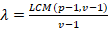
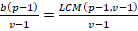
For balanced COD (v, n, p), the requirement is n = λ1v and = λv(v-1)/(p-1) , which implies that λ1(v-1) =λ(v-1) .Suppose that v treatments are tested λ1 times in each period and each treatment is preceded by each other treatments λ2 times, where λ2= b(p-1) v-1 and is known as divisibility condition for existence of balanced design.

A balanced design, which uses the minimum possible no. of units is known as minimal balanced COD.

Theorem 4.1.1 (Afsarinejad, 1990)

The necessary and sufficient conditions for the existence of a minimal balanced CO (v, n, p) with p≤v are n= λ1v and λ1(v-1) =λ(v-1)

Theorem 4.1.2: If vis even, p=4 then, λ=p-1 and b= v-1.

Proof: By definition λ = b (p-1) v-1, Therefore for p = 4, λ = 3, we have b= v-1 and λ=p-1.

Theorem 4.1.3:

For v is odd and p = 3, we always have λ = 1

Proof: By definition

Therefore, for p = 3, λ = 1 we have b= v- 1 2

Results and Discussion

Here we consider that;

By using this information we introduced a new method of getting λ.

Theorem: For v treatments, p periods and b block size, λ is given below;

(3)

Proof:

As we know that

(4)

From eq (3) and (4)

(5)

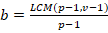(6)

By putting the value of b in eq (4)

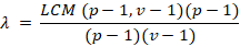
Hence

Example 1:

For 4≤v≤9, p=3

v = 4, p = 3, b = 3

There are 6 possible set of shifts against these parameters,

[1, 1] + [2, 3] + [2, 3]

[1, 1] + [2, 3] + [3, 2]

[1, 1] + [3, 2] + [3, 2]

[1, 2] + [1, 2] + [3, 3]

[1, 2] + [2, 1] + [3, 3]

[2, 1] + [2, 1] + [3, 3]

Now we consider one of the shift to construct the design, we use following sets of shift, [1,1]+[2,3]+[2,3]

Design 1: v = 4, p= 3, b = 3

0	1	2	3	0	1	2	3	0	1	2	3
10	21	32	03	20	31	02	13	20	31	02	13
21	32	03	10	12	23	30	01	12	23	30	01

In Design 1, we used four treatments(v), three periods (p) and block size (b) three. We found that it is Balanced design with λ = 2 and its efficiency is 88.9%. This shows that it contains 88.9 % information out of 100%.

Now we consider the parameters

v=5, p=3, b=4

There are 47 possible set of shifts against these parameters are given below;

[1, 1] + [2, 2] + [3, 3] + [4, 4]

[1, 1] + [2, 2] + [3, 4] + [3, 4]

. . . .

. . . .

. . . .

[3, 1] + [3, 1] + [4, 2] + [4, 2]

By using, [1,1] + [2,2] + [3,3] + [4,4]

Design 2: v=5, p=3, b=4

0	1	2	3	4		0	1	2	3	4
10	21	32	43	04		20	31	42	03	14
21	32	43	04	10		42	03	14	20	31
0	1	2	3	4		0	1	2	3	4
30	41	02	13	24		40	01	12	23	34
13	24	30	41	02		34	40	01	12	23

In Design 2, we used five treatments (v), three periods (p) andblock size (b) four. We found that it is Balanced design with λ = 2 and its efficiency is 96%. This shows that it contains 96 %information out of 100%.

Now we consider the parameters

v = 6, p = 3, b = 5

There are 404 possible set of shifts against these parameters are given below;

[1, 1] + [2, 2] + [3, 4] + [3, 4] + [5, 5]

[1, 1] + [2, 2] + [3, 4] + [3, 5] + [4, 5]

. . . . .

. . . . .

. . . . .

[3, 2] + [4, 1] + [4, 1] + [5, 2] + [5, 3]

By using, [3,2] + [4,1] + [4,1] + [5,2]+ [5,3]

Design 3: v = 6, p = 3, b = 5

0	1	2	3	4	5		0	1	2	3	4	5		0	1	2	3	4	5
30	41	52	03	14	25		40	51	02	13	24	35		40	51	02	13	24	35
53	04	15	20	31	42		54	05	10	21	32	43		54	05	10	21	32	43

0	1	2	3	4	5		0	1	2	3	4	5
50	01	12	23	34	45		50	01	12	23	34	45
15	20	31	42	53	04		25	30	41	52	03	14

In Design 3, we used six treatments(v), three periods (p) and block size (b) five. We found that it is Balanced design with λ =2 and its efficiency is 84 %. This shows that it contains 84 %information out of 100%.

Now we consider the parameters

v=7, p=3, b=3

There are 64 possible set of shifts against these parameters are given below,

[1, 2] + [3, 5] + [4, 6]

[1, 2] + [3, 5] + [6, 4]

. . .

. . .

. . .

[4, 1] + [5, 3] + [6, 2]

[4, 2] + [5, 1] + [6, 3]

By using, [1,2]+[3,5]+[6,4]

Deign 4: v=7, p=3, b=3

0	1	2	3	4	5	6		0	1	2	3	4	5	6
10	21	32	43	54	65	06		30	41	52	63	04	15	26
31	42	53	64	05	16	20		13	24	35	46	50	61	02
0	1	2	3	4	5	6
60	01	12	23	34	45	56
36	40	51	62	03	14	25

In Design 4, we used seven treatments (v), three periods (p) and block size (b) three. We found that it is Balanced design with = 1 and its efficiency is 80 %. This shows that it contains 80 % information out of 100%.

Now we consider the parameters

v=7, p=3, b=6

There are 4027 possible set of shifts against these parameters are given below,

[1, 1] + [2, 2] + [3, 3] + [4, 4] + [5, 5] + [6, 6]

[1, 1] + [2, 2] + [3, 3] + [4, 4] + [5, 6] + [5, 6]

. . . . . .

. . . . . .

. . . . . .

[4, 2] + [4, 2] + [5, 1] + [5, 1] + [6, 3] + [6, 3]

By using, [4,2] + [4,2] + [5,1] + [5,1] + [6,3] + [6,3]

Design 5: v=7, p=3, b=6

0	1	2	3	4	5	6		0	1	2	3	4	5	6
40	51	62	03	14	25	36		40	51	62	03	14	25	36
64	05	16	20	31	42	53		64	05	16	20	31	42	53

0	1	2	3	4	5	6		0	1	2	3	4	5	6
50	61	02	13	24	35	46		50	61	02	13	24	35	46
65	06	10	21	32	43	54		65	06	10	21	32	43	54

0	1	2	3	4	5	6		0	1	2	3	4	5	6
60	01	12	23	34	45	56		60	01	12	23	34	45	56
26	30	41	52	63	04	15		26	30	41	52	63	04	15

In Design 5, we used seven treatments (v ), three periods (p) and block size (b) six. We found that it is Balanced design with = 2 and its efficiency is 81 %. This shows that it contains 81 % information out of 100%.

Now we consider the parameters

v=9, p=3, b=4

There are 960 possible set of shifts against these parameters are given below;

[1; 2] +[3; 4]+ [5; 6]+ [7; 8]

[1; 2]+ [3; 4]+ [5; 6]+ [8; 7]

….

….

[5; 3]+ [6; 4]+ [7; 1]+ [8; 2]

By using, [1,2] + [3,4] + [5,6] + [7,8]

Design 6: v=9, p=3, b=4

0	1	2	3	4	5	6	7	8	0	1	2	3	4	5	6	7	8
10	21	32	43	54	65	76	87	08	30	41	52	63	74	85	06	17	28
31	42	53	64	75	86	07	18	20	73	84	05	16	27	38	40	51	62

0	1	2	3	4	5	6	7	8	0	1	2	3	4	5	6	7	8
50	61	72	83	04	15	26	37	48	70	81	02	13	24	35	46	57	68
25	36	47	58	60	71	82	03	14	67	78	80	01	12	23	34	45	56

In Design 6, we used nine treatments (v), three periods (p) and block size (b) four. We found that it is Balanced design with = 1 and its efficiency is 82 %. This shows that it contains 82 % information out of 100%.

Example 2:

For 4 ≤ v ≤ 7, p = 4

Consider the parameters

v=4, p=4, b=4

There are 6 possible set of shifts against these parameters are given below;

[1; 1; 1]+[2; 1; 2]+[2; 3; 2]+ [3; 3; 3]

[1; 2; 3]+[1; 2; 3]+[1; 2; 3]+ [1; 2; 3]

[1; 2; 3]+[1; 2; 3]+[1; 2; 3]+ [3; 2; 1]

[1; 2; 3]+[1; 2; 3]+[3; 2; 1]+ [3; 2; 1]

[1; 2; 3]+[3; 2; 1]+[3; 2; 1]+ [3; 2; 1]

[3; 2; 1]+[3; 2; 1]+[3; 2; 1]+ [3; 2; 1]

By using, [1,2,3] + [1,2,3] + [1,2,3] + [3,2,1]

Design 7: v=4, p=4, b=4

0	1	2	3	0	1	2	3	0	1	2	3	0	1	2	3
10	21	32	03	10	21	32	03	10	21	32	03	30	01	12	23
31	02	13	20	31	02	13	20	31	02	13	20	13	20	31	02
23	30	01	12	23	30	01	12	23	30	01	12	21	32	03	10

In Design 7, we used four treatments (v), four periods (p) and block size (b) four. We found that it is Balanced design with = 3 and its efficiency is 100 %. This shows that it contains 100 % information out of 100%.

Now we consider the parameters

v=4, p=4, b=5

There are 8 possible set of shifts against these parameters are given below;

[1; 1; 1]+[1; 2; 3] +[2; 1; 2]+ [2; 3; 2]+[3; 3; 3]

[1; 1; 1]+[2; 1; 2]+[2; 3; 2]+[3; 2; 1]+[3; 3; 3]

.....

.....

.....

[3; 2; 1]+[3; 2; 1]+[3; 2; 1]+[3; 2; 1]+[3; 2; 1]

[1; 1; 1]+[1; 2; 3]+[2; 1; 2]+[2; 3; 2]+[3; 3; 3]

[1; 1; 1]+[2; 1; 2]+[2; 3; 2]+[3; 2; 1]+[3; 3; 3]

.....

.....

.....

[3; 2; 1]+[3; 2; 1]+[3; 2; 1]+[3; 2; 1]+[3; 2; 1]

Design 8: v=4, p=4, b=5

0	1	2	3		0	1	2	3		0	1	2	3
10	21	32	03		20	31	02	13		20	31	02	13
21	32	03	10		32	03	10	21		12	23	30	01
32	03	10	21		13	20	31	02		31	02	13	20

0	1	2	3		0	1	2	3
30	01	12	23		30	01	12	23
13	20	31	02		23	30	01	12
21	32	03	10		12	23	30	01

In Design 8, we used four treatments (v), four periods (p) and block size (b) five. We found that it is Balanced design with λ = 5 and its efficiency is 100 %. This shows that it contains 100 % information out of 100%.

Now we consider the parameters

v=4, p=4, b=6

There are 12 possible set of shifts against these parameters are given below;

[1, 1, 1]+[1, 1, 1]+[2, 3, 2]+[2, 3, 2]+[2, 3, 2]+[3, 3, 3]

[1, 1, 1]+[1, 2, 3]+[1, 2, 3]+[2, 1, 2]+[2, 3, 2]+[3, 3, 3]

. . . . . .

. . . . . .

. . . . . .

[3, 2, 1]+[3, 2, 1]+[3, 2, 1]+[3, 2, 1]+[3, 2, 1]+[3, 2, 1]

By using, [1,1,1]+[1,2,3]+[1,2,3]+[2,1,2]+[2,3,2]+ [3,3,3]

Design9: v=4, p=4, b=6

0	1	2	3		0	1	2	3		0	1	2	3
10	21	32	03		10	21	32	03		10	21	32	03
21	32	03	10		31	02	13	20		31	02	13	20
32	03	10	21		23	30	01	12		23	30	01	12

0	1	2	3		0	1	2	3		0	1	2	3
20	31	02	13		20	31	02	13		30	01	12	23
32	03	10	21		12	23	30	01		23	30	01	12
13	20	31	02		31	02	13	20		12	23	30	01

In Design 9, we used four treatments(v), four periods (p) and block size (b) six. We found that it is Balanced design with λ = 5 and its efficiency is 100 %. Which shows that it contains 100 % information out of 100%.

Now we consider the parameters

v=5, p=4, b=4

There are 258 possible sets of shifts against these parameters are given below,

[1, 1, 1] + [2, 2, 2] + [3, 3, 3] + [4, 4, 4]

[1, 1, 1] + [2, 4, 3] + [2, 4, 3] + [2, 4, 3]

. . . .

. . . .

. . . .

[3, 3, 3] + [4, 2, 1] + [4, 2, 1] + [4, 2, 1]

By using, [1,1,1] + [2,4,3] + [2,4,3] + [2,4,3]

Design10: v=5, p=4, b=4

0	1	2	3	4		0	1	2	3	4
10	21	32	43	04		20	31	42	03	14
21	32	43	04	10		12	23	34	40	01
32	43	04	10	21		41	02	13	24	30

0	1	2	3	4		0	1	2	3	4
20	31	42	03	14		20	31	42	03	14
12	23	34	40	01		12	23	34	40	01
41	02	13	24	30		41	02	13	24	30

In Design 10, we used five treatments (v ), four periods (p) and block size (b) four. We found that it is Balanced design with = 3 and its efficiency is 96 %. This shows that it contains 96 % information out of 100 %.

Now we consider the parameters

v=7, p=4, b=2

There are 132 possible set of shifts against these parameters are given below

[1, 2, 3] + [4, 5, 6]

[1, 2, 3] + [4, 6, 5]

. .

. .

. .

[5, 4, 2] + [6, 3, 1]

By using, [1,2,3] + [4,6,5]

Design11: v=7, p=4, b=2

0	1	2	3	4	5	6		0	1	2	3	4	5	6
10	21	32	43	54	65	06		40	51	62	03	14	25	36
31	42	53	64	05	16	20		34	45	56	60	01	12	23
63	04	15	26	30	41	52		13	24	35	46	50	61	02

In Design 11, we used seven treatments(v), four periods (p) and block size (b) two. We found that it is Balanced design with λ = 3 and its efficiency is 89 %. Which shows that it contains 89 % information out of 100 %?

Now we consider the parameters

v=7, p=4, b=4

There are 26601 possible set of shifts against these parameters are given below;

[1; 1; 2]+[2; 3; 3]+[4; 4; 5]+[5; 6; 6]

[1; 1; 2]+[2; 3; 3]+[4; 4; 5]+[6; 5; 6]

....

....

....

[5; 4; 2]+[5; 4; 2]+[6; 3; 1]+[6; 3; 1]

By using, [1,1,2] + [2,3,3] +[4,4,5] + [6,5,6]

Design 12: v=7, p=4, b=4

0	1	2	3	4	5	6		0	1	2	3	4	5	6
10	21	32	43	54	65	06		20	31	42	53	64	05	16
21	32	43	54	65	06	10		52	63	04	15	26	30	41
42	53	64	05	16	20	31		15	26	30	41	52	63	04

0	1	2	3	4	5	6		0	1	2	3	4	5	6
40	51	62	03	14	25	36		60	01	12	23	34	45	56
14	25	36	40	51	62	03		46	50	61	02	13	24	35
61	02	13	24	35	46	50		34	45	56	60	01	12	23

In Design 12, we used seven treatments(v), four periods (p) and block size (b) four. We found that it is Balanced design with λ = 3 and its efficiency is 64 %. Which shows that it contains 64 % information out of 100 %.

Now we consider the parameters

v=4, p=5, b=3

There are 66 possible set of shifts against these parameters are given below;

[1, 1, 1, 2] + [1, 2, 3, 3] + [2, 3, 2, 3]

[1, 1, 1, 2] + [1, 2, 3, 3] + [2, 3, 3, 2]

. . .

. . .

. . .

[3, 2, 1, 1] + [3, 2, 1, 1] + [3, 2, 3, 2]

By using, [1,1,1,2]+ [1,2,3,3] + [2,3,3,2]

Design13: v=4, p=5, b=3

0	1	2	3		0	1	2	3		0	1	2	3
10	21	32	03		10	21	32	03		20	31	02	13
21	32	03	10		31	02	13	20		12	23	30	01
32	03	10	21		23	30	01	12		01	12	23	30
13	20	31	02		12	23	30	01		20	31	02	13

In Design 13, we used four treatments(v), five periods (p) and block size (b) three. We found that it is Balanced design with λ = 3 and its efficiency is 86 %. Which shows that it contains 86 % information out of 100 %.

Large Parameters

The available specifications of the present day computers are not enough to run the software. For large parameters, basic matrix to generate shift contains billions of rows. e.g., v=9, p=4, b=4, basic generated matrix contains more than one billion rows, which is very difficult task for the present day computers to manipulate. These calculations may possible on clusters and super computers. So, further work in this regard will be subject of future interest.

Lemma

There exists

p = 3, b = v - 1 for v = even and b= (v-1)/2, for v=odd

Example 3: For p = 3,9 ≤ v ≤ 22

Table 3: p = 3,9 ≤ v ≤ 22

v	p	Set of Shifts
9	3	[1; 2] + [3; 4] + [5; 6] + [7; 8]
10	3	[1; 2] + [3; 4] + [5; 6] + [7; 8] + [9; 2] + [3; 1] + [5; 4] + [7; 6] + [8; 9]
11	3	[1; 2] + [3; 4] + [5; 6] + [7; 8] + [9; 10]
12	3	[1; 2] + [3; 4] + [5; 6] + [7; 8] + [9; 10] + [11; 2] + [1; 3] + [4; 5] + [6; 7] + [8; 9] + [10; 11]
13	3	[1; 2] + [3; 4] + [5; 6] + [7; 8] + [9; 10] + [11; 12]
14	3	[1; 2] + [3; 4] + [5; 6] + [7; 8] + [9; 10] + [11; 12] + [13; 2] + [1; 3] + [4; 5] + [6; 7] + [8; 9] + [10; 11] + [12; 13]
15	3	[1; 2] + [3; 4] + [5; 6] + [7; 8] + [9; 10] + [11; 12] + [13; 14]
16	3	[1; 2] + [3; 4] + [5; 6] + [7; 8] + [9; 10] + [11; 12] + [13; 14] + [15; 2] + [1; 3] + [4; 5] + [6; 7] + [8; 9] + [10; 11] + [12; 13] + [14; 15]
17	3	[1; 2] + [3; 4] + [5; 6] + [7; 8] + [9; 10] + [11; 12] + [13; 14] + [15; 16]
18	3	[1; 2] + [3; 4] + [5; 6] + [7; 8] + [9; 10] + [11; 12] + [13; 14] + [15; 16] + [17; 2] + [1; 3] + [4; 5] + [6; 7] + [8; 9] + [10; 11] + [12; 13] + [14; 15] + [16; 17]
19	3	[1; 2] + [3; 4] + [5; 6] + [7; 8] + [9; 10] + [11; 12] + [13; 14] + [15; 16] + [17; 18]
20	3	[1; 2] + [3; 4] + [5; 6] + [7; 8] + [9; 10] + [11; 12] + [13; 14] + [15; 16] + [17; 18] + [19; 2] + [1; 3] + [4; 5] + [6; 7] + [8; 9] + [10; 11] + [12; 13] + [14; 15] + [16; 17] + [18; 19]
21	3	[1; 2] + [3; 4] + [5; 6] + [7; 8] + [9; 10] + [11; 12] + [13; 14] + [15; 16] + [17; 18] + [19; 20]
22	3	[1; 2] + [3; 4] + [5; 6] + [7; 8] + [9; 10] + [11; 12] + [13; 14] + [15; 16] + [17; 18] + [19; 20] + [21; 2]+[1; 3]+[4; 5]+[6; 7]+[8; 9]+[10; 11]+[12; 13]+[14; 15]+[16; 17]+[18; 19]+[20; 21]

Example 4:

For p = 4,9 ≤ v ≤ 22

Table 4: p = 4,9 ≤ v ≤ 22

v	p	Set of Shifts
9	4	[1; 2; 3] + [4; 6; 5] + [7; 8; 2] + [1; 3; 4] + [5; 6; 7] + [8; 2; 1] + [3; 4; 5] + [6; 7; 8] + [1; 2; 3] + [4; 6; 5] + [7; 8; 9]
10	4	[1; 2; 3] + [4; 6; 5] + [7; 8; 9]
11	4	[1; 2; 3] + [4; 5; 7] + [6; 8; 9] + [10; 2; 1] + [3; 4; 5] + [6; 7; 8] + [9; 10; 2] + [3; 1; 4] + [5; 7; 6] + [8; 9; 10]
12	4	[1; 2; 3] + [4; 5; 7] + [6; 8; 9] + [10; 11; 2] + [1; 3; 4] + [5; 6; 7] + [8; 9; 10] + [11; 2; 1] + [3; 4; 5] + [6; 7; 8] + [9; 10; 11
13	4	[1; 2; 3] + [4; 5; 7] + [6; 8; 9] + [10; 11; 12]
14	4	[1; 2; 3] + [4; 5; 6] + [7; 8; 9] + [10; 11; 12] + [13; 2; 1] + [3; 4; 5] + [6; 7; 8] + [9; 10; 11] + [12; 13; 2] + [1; 3; 4] + [5; 6; 7] + [8; 9; 10] + [11; 12; 13]
15	4	[1; 2; 3] + [4; 5; 6] + [7; 8; 9] + [10; 11; 12] + [13; 14; 2] + [1; 3; 4] + [5; 6; 7] + [8; 9; 10] + [11; 12; 13] + [14; 2; 1] + [3; 4; 5] + [6; 7; 9] + [8; 10; 11] + [12; 13; 14]
16	4	[1; 2; 3] + [4; 5; 6] + [7; 8; 9] + [10; 11; 12] + [13; 14; 15]
17	4	[1; 2; 3] + [4; 5; 6] + [7; 8; 10] + [9; 11; 12] + [13; 14; 15] + [16; 2; 1] + [3; 4; 5] + [6; 7; 8] + [9; 10; 11]+[12; 13; 14]+[15; 16; 2]+[1; 3; 4] +[5; 6; 7]+[8; 10; 9]+[11; 12; 13]+[14; 15; 16]
18	4	[1; 2; 3] + [4; 5; 6] + [7; 8; 9] + [10; 11; 12] + [13; 14; 15] + [16; 17; 2] + [1; 3; 4] + [5; 6; 7] + [8; 9; 10] + [11; 12; 13] + [14; 15; 16] + [17; 2; 1] + [3; 4; 5] + [6; 7; 8] + [9; 10; 11] + [12; 13; 14] + [15; 16; 17]
19	4	[1; 2; 3] + [4; 5; 6] + [7; 8; 9] + [10; 11; 12] + [13; 14; 15] + [16; 17; 18]
20	4	[1; 2; 3]+[4; 5; 6]+[7; 8; 9]+[10; 11; 12]+[13; 14; 15]+[16; 17; 18] +[19; 2; 1]+[3; 4; 5]+ [6; 7; 8]+[9; 10; 11]+[12; 13; 14]+[15; 16;17] +[18; 19; 2]+[1; 3; 4]+[5; 6; 7]+[8; 9; 10]+ [11; 12; 13] + [14; 15; 16]+ [17; 18; 19]
21	4	[1; 2; 3]+[4; 5; 6]+[7; 8; 9]+[10; 12; 11]+[13; 14; 15]+[16; 17; 18] +[19; 20; 2]+[1; 3; 4]+ [5; 6; 7]+[8; 9; 10]+[11; 12; 13]+[14; 15;16]+[17; 18; 19]+[20; 2; 1]+[3; 4; 5]+[6; 7; 8]+ [9; 10; 11] + [12; 13; 14] + [15; 16; 17] + [18; 19; 20]
22	4	[1; 2; 3] + [4; 5; 6] + [7; 8; 9] + [10; 11; 12] + [13; 14; 15] + [16; 17; 18] + [19; 20; 21]

Example 5:

For p = 5,9 ≤ v ≤ 15

Table 5: p = 5,9 ≤ v ≤ 15

v	p	Set of Shifts
9	5	[1; 2; 3; 4] + [5; 6; 7; 8]
10	5	[1; 2; 3; 5]+[7; 6; 8; 4]+[9; 2; 1; 3]+[4; 5; 6; 7]+[8; 9; 2; 1]+[3; 4; 5; 6] + [7; 8; 9; 2] + [1; 3; 4; 5] + [6; 7; 8; 9]
11	5	[1; 2; 3; 4] + [7; 6; 8; 5] + [9; 10; 2; 1] + [3; 4; 5; 7] + [6; 8; 9; 10]
12	5	[1; 2; 3; 4] + [7; 6; 8; 5] + [9; 10; 11; 2] + [3; 1; 4; 5] + [6; 7; 8; 9] + [10; 11; 2; 1] + [3; 6; 5; 4] + [7; 8; 9; 10] + [11; 2; 1; 3] + [4; 5; 6; 7] + [8; 9; 10; 11]
13	5	[1; 2; 3; 4] + [5; 6; 8; 7] + [9; 10; 11; 12]
14	5	[1; 2; 3; 4] + [7; 6; 5; 8] + [9; 10; 11; 12] + [13; 2; 1; 3] + [4; 5; 6; 7] +[8; 9; 10; 11] + [12; 13; 2; 1] + [3; 4; 5; 6] + [7; 8; 9; 10] + [11; 12; 13; 2] +[1; 3; 4; 5] + [6; 7; 8; 9] + [10; 11; 12; 13]
15	5	[1; 2; 3; 4] + [7; 6; 8; 5] + [9; 10; 11; 12] + [13; 14; 2; 1] + [3; 4; 5; 6] +[8; 9; 10; 7] + [11; 12; 13; 14]

Balanced cross over design with p < v

To construct p < v, we will select the designs which (i) gave off diagonal elements of L matrix, which were as equal as possible, (ii) gave off-diagonal elements of NN 0 which were as equal as possible and (iii) gave off-diagonal elements of the NM 0 matrix which were as equal as possible. Then we selected the design which had the highest efficiency.

However, in these designs, the numbers of periods often exceed the numbers of treatments to be compared. In some experiments, it may be difficult to accommodate a large number of periods and so one may prefer designs with p < v. Patterson (1952) was probably the first to give systematic methods of construction for designs with p < v. Freeman (1959), Patterson and Lucas (1962), Atkinson (1966), Hedayat and Afsarinejad (1975), Constantine and Hedayat (1982), Afsarinejad (1983; 1985) and Stufken (1991) also considered designs with p < v.

Balanced Cross Over Deign with p < v

Now we consider the case where p < v, Jones and Kenward (1989) stated that having p < v useful in order to increase the efficiency of the estimation of the carry-over effects, as well as improving the efficiency of direct effects.

Series 1: v = 5, p = 2i - 1 for i=2,3,..…

Where, λ = i – 1,

Table 1:v = 5, p = 2i - 1

i	p	Set of Shifts
2	3	[1; 2] + [3; 4]
3	5	[1; 2; 4; 3] + [1; 2; 4; 3]
4	7	[1; 2; 4; 3; 1; 2] +[3; 4; 1; 2; 4; 3]
5	9	[1; 2; 4; 3; 1; 2; 4; 3]+[1; 2; 4; 3; 1; 2; 4; 3]
6	11	1; 2; 4; 3; 1; 2; 4; 3; 1; 2]+[3; 4; 1; 2; 3; 4; 1; 2; 4; 3]

Series 2: v = 5, p = 2i - 1 for i=3,5,7,..…

Where λ = (i - 1)/2, b=1

Table 2: v = 5, p = 2i - 1

i	p	Set of Shifts
3	5	[1; 2; 3; 4]
5	9	[1; 2; 4; 3; 1; 2; 4; 3]
7	13	[1; 2; 4; 3; 1; 2; 4; 3; 1; 2; 4; 3]
9	17	[1; 2; 4; 3; 1; 2; 4; 3; 1; 2; 4; 3]
11	21	[1; 2; 4; 3; 1; 2; 4; 3; ; 1; 2; 4; 3; 1; 2; 4; 3; 1; 2; 4; 3]

Series 3:

v =i, p = 3i-1 for i=2,3,4,..…

Where λ =3, b=v-1

Table 3: v =i, p = 3i-1

i	p	Set of Shifts
2	5	[1; 2; 4] + [3; 1; 2] + [3; 4; 2] + [1; 3; 4]
3	8	8 [1; 2; 3] +[ 4; 5; 6] + [7; 2; 1] + [3;4;5] + [6; 7; 2] + [1; 3; 5] + [4; 6;7]
4	11	[1; 2; 3]+[4; 5; 7]+[6; 8; 9]+[10; 2; 1]+[3; 4; 5] + [6; 7; 8]+[9; 10; 2]+[1; 3; 4]+[5; 7; 6]+[8; 9; 10]
5	14	[1; 2; 3] + [4; 5; 7] + [6; 9; 8] + [10; 11; 12] + [13; 2; 1] + [3; 4; 5] + [6; 7; 8] + [9; 10; 11] + [12; 13; 2] + [1; 3; 4] + [5; 6; 7] + [8; 9; 10] + [11; 12; 13]

Series 4:

v =4i, p = 3 for i=2,3,4,..…

Where λ =1,b=2i-1

Table 4: v =4i, p = 3

i	v	Set of Shifts
2	7	[1; 2] + [3; 5] + [4; 6]
3	11	[1; 2] + [3; 4] + [5; 7] + [6; 8] + [9; 10]
4	15	[1; 2] + [3; 4] + [5; 6] + [7; 9] + [8; 10] + [11; 12] + 13; 14]
5	19	[1; 2]+[3; 4]+[5; 6]+[7; 8]+[9; 11]+[10; 12]+[13; 14]+[15; 16]+[17; 18]
6	23	[1; 2] + [3; 4] + [5; 6] + [7; 8] + [9; 10] + [11; 13] + [12; 14] + [15; 16] +[17; 18] + [19; 20] + [21; 22]
7	27	[1; 2] + [3; 4] + [5; 6] + [7; 8] + [9; 10] + [11; 12] + [13; 15] + [14; 16] +[17; 18] + [19; 20] + [21; 22] + [23; 24] + 25; 26]
8	31	[1; 2] + [3; 4] + [5; 6] + [7; 8] + [9; 10] + [11; 12] + [13; 14] + [15; 17] +[16; 18] + [19; 20] + [21; 22] + [23; 24] + [25; 26] = [27; 28] + [29; 30]
9	35	[1; 2] + [3; 4] + [5; 6] + [7; 8] + [9; 10] + [11; 12] + [13; 14] + [15; 16] +[17; 18] + [19; 20] + [21; 22] + [23; 24] + [25; 26] + [27; 29] + [28; 30] +[31; 32] + [33; 34]
10	39	[1; 2] + [3; 4] + [5; 6] + [7; 8] + [9; 10] + [11; 12] + [13; 14] + [15; 16] +[17; 18] + [19; 20] + [21; 22] + [23; 24] + [25; 26] + [27; 28] + [29; 30] +[31; 32] + [33; 34] + [35; 36] + [37; 38]

Series 5:

v =2,4,6,8,…………..p = 3,b=v-1

thenλ =2,

For small parameters MATLAB is used,

Table 5: v =2,4,6,8,…………..p = 3,

v	Set of Shifts
10	[1, 2] + [3, 4] + [5, 6] + [7, 8] + [9, 2] + [1, 3] + [4, 5] + [6, 7] + [8, 9]
12	[1, 2] + [3, 4] + [5, 6] + [7, 8] + [11, 2] + [1, 3] + [4, 5] + [6, 7] + [8, 9] + [10, 11]
14	[1, 2] + [3, 4] + [5, 6] + [7, 8] + [9, 10] + [11, 12] + [13, 2] + [1, 3] + [4, 5] +[6, 7] + [8, 9] + [10, 11] + [12, 13]
16	[1, 2] + [3, 4] + [5, 6] + [7, 8] + [9, 10] + [11, 12] + [13, 2] + [1, 3] + [4, 5] +[6, 7] + [8, 9] + [10, 11] + [12, 13] + [14, 15]
18	[1, 2] + [3, 4] + [5, 6] + [7, 8] + [9, 10] + [11, 12] + [13, 14] + [15,16] + [17, 2] +[1, 3] + [4, 5] + [6, 7] + [8, 9] + [10, 11] + [12, 13] + [14, 15] + [16, 17]
20	[1, 2]+[3, 4]+[5, 6]+[7, 8]+[9, 10]+[11, 12]+[13, 14]+[15, 16] +[17, 18] + [19, 2]+[1, 3]+[4, 5]+[6, 7]+[8, 9]+[10, 11]+[12, 13] +[14, 15]+[16, 17] + [18, 19]

Series 6:

v =4i-1, p = 3, b=(v-1)/2, i=2,3,4,……, and λ = 1

Table 6: v =4i-1, p = 3

v	Set of Shifts
5	[1; 2] + [3; 4]
9	[1, 2] + [3, 4] + [5, 6] + [7, 8]
13	[1, 2] + [3, 4] + [5, 6] + [7, 8] + [9, 10] + [11, 12]
17	[1, 2] + [3, 4] + [5, 6] + [7, 8] + [9, 10] + [11, 12] + [13, 14] + [15, 16]
21	[1, 2]+[3, 4]+[5, 6]+[7, 8]+[9, 10]+[11, 12]+[13, 14]+[15, 16]+[17, 18]+[19, 20]
25	[1, 2]+[3, 4]+[5, 6]+[7, 8]+[9, 10]+[11, 12]+[13, 14]+[15, 16]+[17, 18]+[19, 20] + [21, 22] + [23, 24]

Series 7:

v =3,5,7,………..p = 3,b=(v-1)/2, and λ = 1 ,

Table 7: v =3,5,7,………..p = 3

V	Set of Shifts
9	[1; 2] + [3; 4] + [5; 6] + [7; 8]
11	[1; 2] + [3; 4] + [5; 6] + [7; 8] + [9; 10]
13	[1; 2] + [3; 4] + [5; 6] + [7; 8] + [9; 10] + [11; 12]
15	[1; ; 2] + [3; 4] + [5; 6] + [7; 8] + [9; 10] + [11; 12] + [13; 14]
17	[1; 2] + [3; 4] + [5; 6] + [7; 8] + [9; 10] + [11; 12] + [13; 14] + [15; 16]
19	[1; 2] + [3; 4] + [5; 6] + [7; 8] + [9; 10] + [11; 12] + [13; 14] + [15; 16] + [17; 18]
21	[1; 2] + [3; 4] + [5; 6] + [7; 8] + [9; 10] + [11;12] + [13;14] + [15; 16] + [17; 18] + [19; 20]

Series 8:

v =9,13,15,17,………..p = 4,

Table 8: v =9,13,15,17,………..p = 4

v	Set of Shifts
9	[1; 2; 3] + [4; 6; 5] + [7; 8; 2] + [1; 3; 4] + [5; 6; 7] + [8; 2; 1] + [3; 4; 6] + [5; 7; 8]
11	[1; 2; 3] + [4; 5; 7] + [6; 8; 9] + [10; 2; 1] + [3; 4; 5] + [6; 7; 8] + [9; 10; 2] + [1; 3; 4] + [5; 7; 6] + [8; 9; 10]
13	[1; 2; 3] + [4; 5; 6] + [7; 8; 9] + [10; 11; 12]
15	[1; 2; 3] + [4; 5; 6] + [7; 9; 8] + [10; 11; 12] + [13; 14; 2] + [1; 3; 4] + [5; 6; 8] + [9; 10; 11] + [12; 13; 14] + [7; 2; 1] + [3; 4; 5] + [6; 7; 9] + [8; 10; 11] + [2; 13; 14]
17	[1; 2; 3] + [4; 5; 6] + [7; 8; 10] + [9; 11; 12] + [13; 14; 15] + [16; 2; 1] + [3; 4; 5] + [6; 7; 8] + [9; 10; 11]+[12; 13; 14]+[15; 16; 2]+[1; 3; 4] +[5; 6; 7]+[8; 10; 9]+[11; 12; 13]+[14; 15; 16]
19	[1; 2; 3] + [4; 5; 6] + [7; 8; 9] + [10; 11; 12] + [13; 14; 15] + [16; 17; 18]
21	[1; 2; 3]+[4; 5; 6]+[7; 8; 9]+[10; 11; 12]+[13; 14; 15]+[16; 17; 18] +[19; 20; 2]+[1; 3; 4]+ [5; 6; 7]+[8; 9; 10]+[11; 12; 13]+[14; 15; 16] +[17; 18; 19]+[20; 2; 1]+[3; 4; 5]+[6; 7; 9]+ [8; 10; 12] + [11; 13; 14] + [15; 16; 17] + [18; 19; 20]
23	[1; 2; 3] + [4; 5; 6] + [7; 8; 9] + [10; 11; 13] + [12; 14; 15] + [16; 17; 18] + [19; 20; 21] + [22; 2; 1] + [3; 4; 5] + [6; 7; 8] + [9; 10; 11] + [12; 13; 14] + [15; 16; 17] + [18; 19; 20] + [21; 22; 2]+[1; 3; 4]+[5; 6; 7]+[8; 9; 10]+[11; 13; 12] +[14; 15; 16]+[17; 18; 1]+[20; 21; 22]

Analysis of Cross Over Design

The crossover design has n treatment sequence group and ri subjects in the ith group. There are v treatments and each group of subjects receives treatments in a different order for p treatments periods.

Example 5:

Twelve wheat types were available for the study. Each of the three fertilizers were spread to the wheat in one of the six possible sequences. Each fertilizer in each sequence was spread to two wheat types for 30 days. The wheat types were given a period of 21 days to adapt to a fertilizer change before any data were collected.

The coefficient calculated for each wheat type on each fertilizer is shown in following table. The given coefficient indicate the per cent of fertilizer absorb by wheat field.

Sequence

	1			2			3
Wheat types		1	2		3	4		5	6
Period 1	(A)	50	55	(B)	44	51	(C)	35	41
Period 2	(B)	61	63	(C)	42	45	(A)	55	56
Period 3	(C)	53	57	(A)	57	59	(B)	47	50

	4			5			6
Wheat types		7	8		9	10		11	12
Period 1	(A)	54	58	(B)	50	55	(C)	41	46
Period 2	(C)	48	51	(A)	57	59	(B)	56	58
Period 3	(B)	51	54	(C)	51	55	(A)	58	61

Now we will apply our method of construction upon this data and then we will have its analysis of variance (ANOVA). We will apply [1,1], [1,1],[2,2], [2,2] set of shifts to construct the new design.

Table: Analysis of Variance Table for a Cross Over Design with n sequences, p periods, v treatments and ri subjects in the sequence

Source of Variation	Degrees of Freedom	Sum of Squares	Mean Squares
Between Subject :
Sequence	n-1	SSS	MSS
Subjects with in Sequence	N-n	SSW	MSW
With in Subjects:
Periods	p-1	SSP	MSP
Treatments (direct)	t-1	SST	MST
Treatments (Carry over e ect)	t-1	SSC	MSC
Error	(N-1)(p-1)-2(t-1)	SSE	MSE
Total	Np-1	SSTotals

Source of Variation	Degrees of freedom	Sum of Squares	Mean Squares
Between Subject :
Sequence	5	331.67	66.33
Subjects with in Sequence	6	114.33	19.06
With in Subjects:
Periods	2	288.17	144.08
Treatments (direct)	2	559.5	279.75*
Error	18	161.96	9
Total		1474

This ANOVA will be the same, whatever set of shifts are applied. The concept we have developed will enhance the choice in cyclic shifts. Which will be really helpful for the policy setters.

Conclusions and Recommendations

In this article, we are concerned with the construction of CODs by using MATLAB. Many of the new designs have been introduced.

In the present study, balanced cross over design has been modified by giving all possible set of shifts. The advantage of having all possible shifts is that one can use value of his/her own requirement. Further we are working on the efficiency of these shifts. This will make us able to select one shift which will give the efficient results.

Further we suggest that by using simulation method one can generate the data set and apply these shifts upon them. This will be the great thing to do which willopen the new door in research.

Cross over designs provide an economy of resources when a limited number of units are available for the study. Most commonly, cross over designs are used with human and animal subjects. The expense of maintaining large animals and the difficulties in recruiting adequate numbers of human subject to achieve sufficient replication make cross over designs more attractive since they require fewer units for an equal number of replication.
In above example, roughage diets are balanced row-column design. The periods and steers are the rows and columns of the design. Each of the roughage diet occur one time in each steers and four times in each period of the design. Efficiencies of these shifts can be found in further work.

Novelty Statement

In this research, MATLAB to construct cross over design was used. This is a novel innovation enabling possible shift in one click.

Author’s Contribution

Aasma Younas: Developed the computer program and wrote draft of the manuscript.

Ijaz Iqbal: Designed the idea of the study.

Atif Akbar: Helped in proofreading of the manuscript.

Conflict of interest

The authors have declared no conflict of interest.

References

Afsarinejad, K. 1983. Balanced repeated measuremets designs. Biometrika, 70: 199–204. https://doi.org/10.1093/biomet/70.1.199

Afsarinejad, K. 1985. Optimal repeated measurements designs. Statistics, 16: 563–568. https://doi.org/10.1080/02331888508801892

Atkinson, G.F. 1966. Designs for sequences of treatments with carry-over effects. Biometrics, 22: 292–309. https://doi.org/10.2307/2528520

Bishop, S.H. and Jones, B. 1984. A review of higher order crossover designs. J. Appl. Stat., 11(1):29-50. https://doi.org/10.1080/02664768400000005

Bose, M. and A. Dey. 2009. Optimal Crossover Designs. Hackensack, NJ: World Scientific. https://doi.org/10.1142/6878

Cochran, W.G. 1939. Long term agricultural experiments. J. Roy. Statist. Soc. Suppl., 6:104-148. https://doi.org/10.2307/2983686

Cochran. W.G., Autrey, K.M. and Canon, C.Y. 1941. A double change over design for dairy cattle feeding experiments. J. Diary Sci., 24:937-951. https://doi.org/10.3168/jds.S0022-0302(41)95480-2

Constantine, G. and A. Hedayat. 1982. A construction of repeated measurements designs with balance for residual effects. J. Statist. Plann. Inference, 6: 153–164. https://doi.org/10.1016/0378-3758(82)90084-2

Daniyal, M., A. Rashid, F. Shehzad, M.H. Tahir and Zafar, I. 2020. Construction of repeated measurements designs strongly balanced for residual effects, Communications in Statistics – Theory and Method., 49(17): 4288-4297. https://doi.org/10.1080/03610926.2019.1599019

Davis, A.W. and W.B. Hall. 1969. Cyclic change-over designs. Biometrika., 56: 283-293.

Freeman, G.H. 1959. The use of the same experimental material for more than one set of treatments. Appl. Statist., 8: 13–20. https://doi.org/10.2307/2985808

Patterson, H.D. and Williams. 1976. A new class of resolvable incomplete block design. Biometrika, 63 (01): 83-92. https://doi.org/10.1093/biomet/63.1.83

Hedayat, A.S. and Yang, M. 2003. Universal optimality of balanced uniform crossover designs. Ann. Statist., 31: 978–983. https://doi.org/10.1214/aos/1056562469

Hedayat, A. and K. Afsarinejad. 1975. Repeated measurements designs, I. In A Survey of Statistical Designs and Linear Models (J.N. Srivastava, Ed.). Amsterdam: North-Holland, pp. 229–242.

Iqbal, I. 1991. Construction of Experimental Designs Using Cyclic Shifts. Ph.D. thesis, University of Kent at Canterbury, UK.

Iqbal, I. and Jones, B. 1994. Efficient repeated measurements designs with equal and unequal period sizes. J. Statist. Plann. Infer., 42 (1-2):79-88. https://doi.org/10.1016/0378-3758(94)90190-2

Jarrett, R.G.  and W.B. Hall. 1978. Generalized cyclic incomplete block designs. Biometrika., 65: 397-401. https://doi.org/10.1093/biomet/65.2.397

John, J.A. 1981. Efficient Cyclic Designs. J. Royal Statist. Soc., 43 (1): 1-14. https://doi.org/10.1111/j.2517-6161.1981.tb01151.x

John, J.A., Wolock, F.W. and David, H.A. 1972.Cyclic Designs. U.S. Department of Commerce, National Bureau of Standards, 62:1-72

Lamacraft, R.R. and Hall, W.B. 1982. Tables of cyclic incomplete block designs: Austral. J. Statist., 24(3): 350-360. https://doi.org/10.1111/j.1467-842X.1982.tb00840.x

Park, D.K., M. Bose, W.I. Notz and A.M. Dean. 2011. Efficient crossover designs in the presence of interactions between direct and carry-over treatment effects. J. Statist. Plann. Infer., 141: 846–860. https://doi.org/10.1016/j.jspi.2010.08.005

Patterson, H.D. 1952. The construction of balanced designs for experiments involving sequences of treatments. Biometrika, 39: 32–48. https://doi.org/10.1093/biomet/39.1-2.32

Patterson, H.D. and H.L. Lucas. 1962. Change-over Designs. North Carolina Agric. Exp. Station Tech. Bull., No. 147.

Roy, B.K. 1988. Construction of strongly balanced uniform repeated measurements designs . J. Statist. Plann. Infer., 19 : 341 – 348. https://doi.org/10.1016/0378-3758(88)90041-9

Sen, M. and Mukerjee, R. 1987. Optimal repeated measurements designs under interaction. J. Statist. Plann. Infer., 17: 81 – 91. https://doi.org/10.1016/0378-3758(87)90102-9

Senn, S.J. 2000. Crossover design. In Encyclopaedia of Biopharmaceutical Statistics (S. C. Chow, Ed.). New York: Marcel Dekker. pp. 142–149.

Stufken, J. 1991. Some families of optimal and efficient repeated measurements designs. J. Statist. Plann. Infer., 27: 75–83. https://doi.org/10.1016/0378-3758(91)90083-Q

Tudor, G.E., Koch, G.G. and Catellier, D. 2000. Statistical methods for crossover designs in bio environmental and public health studies. In Sen, P.K. and Rao, C.R., editors, Handbook of Statistics, Elsevier Science B.V., 18: 571-614. https://doi.org/10.1016/S0169-7161(00)18022-8

Wellek, S. and Blettner, M. 2012. Use of crossover design in clinical trials. Dtsch Arztebl Int., 109(15): 276-281. https://doi.org/10.3238/arztebl.2012.0276

Wilk, A. and Kunert, J. 2015. Optimal crossover designs in a model with self and mixed carryover effects with correlated errors. Metrika, 78(2):161–174. https://doi.org/10.1007/s00184-014-0494-8

Williams, E.R. 1949. Experimental designs balanced for the estimation of residual effects of treatments. Austal. J. Sci. Res., A2: 149-168. https://doi.org/10.1071/CH9490149

Yan, Z. 2008. Crossover designs based on type I orthogonal arrays for a self and simple mixed carryover effects models with correlated errors. J. Statist. Plann. Infer., 138:2201-2213. https://doi.org/10.1016/j.jspi.2007.09.010