Research Article

Evaluation of Carcass Characteristics of Japanese Quail Using Principal Component Analysis (PCA)

Fatma Desouki Mohammed Abdallah

Department of Animal Wealth Development, Faculty of Veterinary Medicine, Zagazig University, Egypt.

Received | December 16, 2021; Accepted | January 29, 2022; Published | March 10, 2022

*Correspondence | Fatma Desouki Mohammed Abdallah, Department of Animal Wealth Development, Faculty of Veterinary Medicine, Zagazig University, Egypt; Email: moibho_stat2021@yahoo.com

Citation | Abdallah FDM (2022). Evaluation of carcass characteristics of Japanese quail using principal component analysis (PCA). Adv. Anim. Vet. Sci. 10(4):771-778.

DOI | https://dx.doi.org/10.17582/journal.aavs/2022/10.4.771.778

ISSN (Online) | 2307-8316

Copyright: 2022 by the authors. Licensee ResearchersLinks Ltd, England, UK.

This article is an open access article distributed under the terms and conditions of the Creative Commons Attribution (CC BY) license (https://creativecommons.org/licenses/by/4.0/).

INTRODUCTION

Japanese quail have been used to improve the meat production. Different studies for improving the growth rate and egg production have been performed for Japanese quail to compensate apart of shortage in animal protein (Aggrey et al., 2003).

Many studies in animal and poultry areas such as quail need the measurement of variables of choice to give a suitable characterization of animals or experimental groups, so multivariate methods are applied (Ribeiro et al., 2018). Principal component analysis is a multivariate statistical method of data analysis. It is similar to exploratory factor analysis. It is known as variable-reduction technique which aims to decrease a large group of variables into a small artificial ones known as principle components. These components are uncorrelated and represent most of the variance in the old variables (Bishop et al., 2010). It is firstly known through Karl Pearson followed by Hotelling who predicted different components of different traits of egg production and carcass traits (Shaker and Aziz, 2017; Ukwu et al., 2017). In animal science, it is widely used in many species as follows: In horses, morphometric traits are studied by Pinto et al. (2005). In chicken, different traits studied by Yamaki et al. (2009). Leite et al. (2009) studied eleven quail carcass traits and the results were that only four traits were convenient in his study. Performance traits in Angus cattle are studied by (Pinto et al., 2013). It is found that four principal components of fifteen traits explained 80% of total variance. The relationship between slaughter weight and carcass characteristics is useful in expecting of other body characteristics (Philip and Udeh, 2021).

The significance and advantages of this technique are: less complexity of the data, no repetition and it concentrate on the great variance in the data, and ignore smaller ones so provide restructure of data and decrease messy data (Phillips et al., 2005). Also, there is no need to difficult calculations and this method gives graphical representation of the most common patterns in the data set without any information about groups in the process of reduction (Sodhi and Lal, 2013). Dimension and synchronized dimension reduction method help in finding variables that are characteristic of a group of samples. But its disadvantages are difficulty in evaluating covariance matrix (Phillips et al., 2005) and no accuracy as other reduction method in case of smaller sample size (Sodhi and Lal, 2013).

The objective of the study was to describe the carcass traits using PCA and to predict new carcass measurements derived from this analysis. It lowers a larger set of traits into a smaller set of new traits, known as principle components, which represent most of the variance in the main traits.

MATERIALS AND METHODS

Source of data

Data for this study were obtained from a thesis at the Department of Animal Wealth Development, Faculty of Veterinary Medicine, Zagazig University, Egypt. A total of 720 data values of carcass traits of three lines of Japanese quail were used. The main author for this thesis gave its signed agreement for extracting his data.

These data included three lines of Japanese quail (high body weight, low body weight and random bred control). A sample of thirty birds of each line is selected randomly for this study for measuring different carcass traits (Roushdy, 2014). The online sample size calculator is used to calculate sample size depending on standared deviation, confidence interval, population size and Z scores table.

A sample of 30 birds is randomly selected for each line for eight variales. Then, the total values of data 30 value × 8 variables × 3 lines = 720 data value.

The variables under study (carcass traits) which were measured (gm) as follows:

• Live body weight (gm).
• Body weight at slaughter age (after bleeding) (gm).
• Dressing weight (after bleeding and plucking) (gm).
• Eviscerated carcass weights (empty carcass weight) (gm).
• Weight of the edible giblets (heart, liver, spleen and empty gizzard) (gm).

These carcass traits were measured in the third generation of selection, at 4th week of age, the birds were randomly selected, weighed and then slaughtered, plucked and then carcass was eviscerated.

Statistical analysis

Shapiro-Wilk test of normality for variables was the first step in the analysis process before applying PCA. It tests if the data follow the normal distribution or not.

Model assumption

Before applying PCA, it is important to check four assumptions of it.

1. This technique includes multiple variables. They are interval- ratio level measurement and ordinal variables are very commonly used.
2. Achieving normality and linearity (linear relationship between all variables) depending on scatterplot matrix. If this assumption is not achieved, transformations are applied for interval- ratio level measurement only not with of ordinal data.
3. The sample must be adequate; the number of values is at least of 150 cells or cases (5 to 10 cells for each trait) to be the lowest sample size can be used. The Kaiser-Meyer-Olkin (KMO) used to evaluate if the sample is adequate or not for all data values and for each variable individually.
4. Fitness of data for reduction. Correlations between variables should be adequate to reduce them into a smaller number of components. Bartlett’s test of sphericity is used for this purpose.
5. Absence of outliers is important to avoid its effect on the results.

Mathematical model of PCA

Generally, PCA model is pci=ai1x1+ai2x2+ ……+ aipxp. Then,

y1 or pc1=a11x1+a12x2+ ……+ a1pxp

y2 or pc2=a21x1+a22x2+……+ a2pxp

yp or pcp=ap1x1+ap2x2+..….+ appxp

Where; ai1, ai2, aip are considered the pc coefficients (Everitt et al., 2001).

Bartlett’s test of sphericity

This method tests the hypothesis of no relation between variables. Significant level (P < 0.05) indicates suitability of variables and the analysis can be done.

H0 = R = I

H1= R ≠ I

R= is the correlation matrix

I = is the identity (zero) matrix

Where;

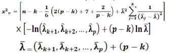
n: sample size; p: total number of eigenvalues; k: number of eigenvalues previously tested; v: represents degrees of freedom with χ2 test statistic, and equals (p - k - 1) (p - k + 2)/2 as explained in (Gouda, 2019).

Kasiser meyer olkin measure of sampling adequacy (MSA)

It measures if the sample adequate or not for a variable Xi. It is the ratio of numerator (sum of squared simple correlation coefficients between factors) and denominator (sum of squared simple correlation coefficients between factors plus partial correlation coefficients of these factors) as in the following equation:

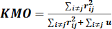
Where; rij is the correlation matrix and u= uij is the partial covariance matrix. MSA measure ranges from 0 to 1, so Kaiser said that KMO of 0.9 considered wonderful, above 0.8 as meritorious, above 0.7 as moderate, above 0.6 as average, above 0.5 as powerless, and below 0.5 as rejected (Gouda, 2019).

Descriptive statistics and other calculations of the carcass traits of each line were calculated using SPSS 21 (2017).

Pearson correlation coefficients among the variables were calculated for each line of Japanese quail and the correlation matrix is calculated as the first step for PCA. Bartlett’s test of sphericity applied to test the identity of correlation matrix (each variable correlated with itself) or a correlation matrix full of zero. Kaiser- Meyer-Olkin (KMO) is used to measure sampling adequacy and the fitness of the data set to PCA. A KMO measure of 0.60 and above is considered appropriate (Eyduran et al., 2010).

Eigenvalues

It is a value that explains the amount of variance of the data and its spread on the line (a measure of explained variance). The eigenvector of the largest eigenvalue is the principal component.

Any factor has eigenvalues more than 1.0, considered an indicator for a factor to be helpful. The eigenvalue less than 1.0, give an indication that the factor gives less information.

RESULTS AND DISCUSSION

Shapiro-Wilk test of normality for carcass traits was non-significant (P value ≥ 0.05) which revealed that the variables are normally distributed and there no need for transformations.

Descriptive statistics of the carcass traits of each line (mean, standard deviation and coefficients of variation) are presented in Table 1.

 

Table 1: Descriptive statistics for body weight and carcass traits in different lines of Japanese quail.

Traits	Mean	Standard deviation	Coefficient of variation
High body weight
Live wt.	167.97	31.08	18.51
Slaughter wt.	162.50	30.63	18.85
Dressing wt.	140.57	26.84	19.09
Carcass wt.	107.57	23.09	21.47
Liver wt.	5.27	1.07	20.30
Gizzard wt.	4.38	1.15	26.26
Heart wt.	1.393	0.34	24.46
Spleen wt.	0.27	0.11	40.74
Low body weight
Live wt.	152.57	28.42	18.63
Slaughter wt.	147.25	28.11	19.08
Dressing wt.	126.66	25.05	19.78
Carcass wt.	94.67	21.79	23.01
Liver wt.	5.04	0.87	17.26
Gizzard wt.	4.12	1.01	24.51
Heart wt.	1.21	0.32	26.45
Spleen wt.	0.17	0.11	64.71
Random bred control
Live wt.	157.41	30.49	19.37
Slaughter wt.	151.88	30.22	19.89
Dressing wt.	131.58	26.98	20.50
Carcass wt.	98.58	21.90	22.21
Liver wt.	5.19	1.09	21.00
Gizzard wt.	4.41	1.48	33.78
Heart wt.	1.25	0.34	27.2
Spleen wt.	0.31	0.12	38.71

 

The correlation coefficients of carcass traits of Japanese quail for different lines were presented in Table 2. The values of correlation coefficient between different traits were moderate to high, and there were few traits showed weak coefficients. These data are suitable for reduction process. These results were in agreement with (Akinsola et al., 2014) who applied principal component analysis on body weight and body measurements in rabbits.

The results of Kaiser-Meyer-Olkin (KMO) and Bartlett’s test of sphericity were showed in Table 3. The KMO values were 0.611, 0.743, and 0.588 for high body weight, low body weight, and random bred control line, respectively. Hair et al. (2010) mentioned that the lowest accepted value for the test was 0.5. Bartlett’s test indicated that the data were suitable for the analysis where P-values < 0.001 were highly significant. This result is in agreement with (Shaker et al., 2019).

The communalities represent estimates of the variance in each trait accounted for by the components as in Table 4. It explained the communalities, where the initial communalities represent the correlation between the variable and all other variables before rotation. If many communalities are less than 0.30, the results become bad because of small sample size. The results showed that all communalities are of good values as follows: It ranged 0.497 (dressing wt)-0.990 (slaughter wt), 0.663 (spleen wt)- 0.854 (carcass wt) and 0.537 (dressing wt)-0.975 (slaughter wt), in high body weight, low body weight and random bred control, respectively. The lowest communality was for dressing wt (0.497) in high body weight line. It was weak in explaining the total variation in the carcass traits of high body weight line.

Table 5 showed that the total variance is divided among the eight possible factors. The total variance explained by the three produced components in high body weight line was (82.193%). This total variance is divided into 53.927% for the first principal component, 15.188% for the second component and the third one was 13.078%. Eigenvalues were 4.314, 1.215 and 1.046 for the first principal component (PC1), the second (PC2) and the third (PC3), respectively.

 

Table 2: Correlation matrix between traits of each line.

Lines		Live wt	Slaughter wt	Dressing wt	Carcass wt	Liver wt	Gizzard wt	Heart wt	Spleen wt
High body weight	Live wt.	1.000
	Slaughter wt.	0.999	1.000
	Dressing wt.	0.497	0.514	1.000
	Carcass wt.	0.554	0.559	0.604	1.000
	Liver wt.	0.275	0.278	0.433	0.662	1.000
	Gizzard wt.	0.510	0.506	0.271	0.525	0.701	1.000
	Heart wt.	0.579	0.579	0.517	0.833	0.527	0.280	1.000
	Spleen wt.	-0.198	-0.205	-0.158	-0.308	-0.033	-0.020	-0.390	1.000
Low body weight	Live wt.	1.000
	Slaughter wt.	0.999	1.000
	Dressing wt.	0.647	0.658	1.000
	Carcass wt.	0.689	0.690	0.684	1.000
	Liver wt.	0.378	0.378	0.441	0.681	1.000
	Gizzard wt.	0.432	0.425	0.317	0.529	0.562	1.000
	Heart wt.	0.698	0.699	0.617	0.827	0.547	0.175	1.000
	Spleen wt.	0.591	0.595	0.683	0.629	0.254	0.235	0.537	1.000
Random bred control	Live wt.	1.000
	Slaughter wt.	0.998	1.000
	Dressing wt.	0.374	0.387	1.000
	Carcass wt.	0.345	0.332	0.556	1.000
	Liver wt.	0.013	-0.013	0.271	0.690	1.000
	Gizzard wt.	0.048	0.044	0.332	0.418	0.387	1.000
	Heart wt.	0.339	0.353	0.487	0.757	0.444	0.234	1.000
	Spleen wt.	-0.197	-0.217	-0.111	-0.171	0.014	0.144	-0.385	1.000

 

Table 3: Kaiser-Meyer-Olkin measure of sampling adequacy (KMO) and Bartlett’s test of sphericity between different lines.

		High body weight	Low body weight	Random bred control
Kaiser Meyer Olkin measure of sampling adequacy		0.611	0.743	0.588
Bartlett's test of sphericity	Approx. Chi-Square	289.458	299.834	222.813
	df	28	28	28
	P-value	0.000**	0.000**	0.000**

 

***P < 0.001= Chi-square value was highly significant.

 

The total variance explained by the two extracted components of low body weight line was 76.429% which divided into (62.504% for the first principal component and 13.925% for the second component). Eigenvalues were 5.000 and 1.114 for the first principal component (PC1), and the second (PC2), respectively.

The total variance explained by the three extracted components was 78.669% for random bred control line. It divided into 42.363% for the first principal component, 22.478% for the second component and 13.827% for the third component. Their Eigenvalues were 3.389, 1.798, and 1.106 for the first principal component (PC1), the second (PC2) and the third (PC3) respectively. Any Eigenvalues lower than 1 means that the factor gives less information than explained one as it is a measure of explained variance.

 

Table 4: Communalities of all traits in each line.

	High body weight		Low body weight		Random bred control
	Initial	Extraction	Initial	Extraction	Initial	Extraction
Live wt.	1.000	0.988	1.000	0.818	1.000	0.963
Slaugt wt.	1.000	0.990	1.000	0.824	1.000	0.975
Dress wt.	1.000	0.497	1.000	0.694	1.000	0.537
Carcas wt.	1.000	0.870	1.000	0.854	1.000	0.871
Liver wt.	1.000	0.925	1.000	0.791	1.000	0.705
Gizzard wt.	1.000	0.760	1.000	0.752	1.000	0.625
Heart wt.	1.000	0.810	1.000	0.718	1.000	0.797
Spleen wt.	1.000	0.736	1.000	0.663	1.000	0.820

 

Table 5: Total variance explained by extracted component scores.

High body weight				Low body weight			Random bred control
Component	Initial eigenvalues			Initial eigenvalues			Initial eigenvalues
	Total	% of variance	Cumulative %	Total	% of variance	Cumulative %	Total	% of variance	Cumulative %
1	4.314	53.927	53.927	5.000	62.504	62.504	3.389	42.363	42.363
2	1.215	15.188	69.115	1.114	13.925	76.429	1.798	22.478	64.841
3	1.046	13.078	82.193	0.714	8.925	85.354	1.106	13.827	78.669
4	0.717	8.965	91.158	0.584	7.301	92.655	0.649	8.107	86.775
5	0.458	5.728	96.886	0.314	3.921	96.576	0.558	6.974	93.750
6	0.175	2.185	99.071	0.203	2.536	99.112	0.351	4.385	98.135
7	0.074	0.923	99.994	0.070	0.879	99.991	0.148	1.850	99.984
8	0.001	0.006	100.000	0.001	0.009	100.000	0.001	0.016	100.000

 

 

Figure 1 showed different scree plots of the number of extracted component for each line, the extracted component was with eigenvalue more than 1 at points of inflexion. High body weight line had three components, low body weight line had two components, and random bred control line had three components.

Table 6 showed rotated component matrix which explains the loading degree (correlation between the components and the traits) in the three lines. In the high body weight line, PC1 had high loadings on live weight (0.962), and slaughter weight (0.961). PC2 had high loadings on liver weight (0.956), gizzard weight (0.752) and carcass weight (0.694). PC3 had high negative loadings for spleen weight (-0.851), and heart weight (0.656).

For low body weight line, PC1 had high loadings (correlation) on slaughter weight (0.869), live weight (0.864), spleen weight (0.813), heart weight (0.799), dressing weight (0.797), and carcass weight (0.722).

PC2 had high loadings on gizzard weight (0.856), liver weight (0.850) and carcass weight (0.578).

For random bred control line, PC1 had high correlation with carcass weight (0.884), liver weight (0.827), heart (0.710), gizzard (0.649) and dressing weight (0.584). PC2 had high correlation with slaughter weight and live weight (0.978, 0.978), respectively. PC3 had high correlation with spleen weight (0.896).

Figure 2 showed the extracted components in each line and the loadings or the variables that correlated to each principal component after varimax rotation.

 

 

CONCLUSION and Recommendations

Depending on the results of this study, the conclusion is that three PC were extracted from eight variables of the high body weight line, two PC were extracted from eight variables of the low body weight line and three PC were extracted from eight variables of random bred control line.

The extracted components could be used as selection criteria for improving next generations. The components could also be used as factor scores for predicting the carcass characters in quail and this improving the production.

ACKNOWLEDGeMENTS

The author wish to express her gratitude to Faculty of Veterinary Medicine/ Zagazig University for supporting this work.

Novelty Statement

This study was firstly applied principle component method on carcass traits of three different lines of Japanese quail.

Conflict of interests

The author has declared no conflict of interest.

REFERENCES

Aggrey SE, Ankra GA, Marks HL (2003). Effect of long term divergent selection on growth characteristics in Japanese quails. Poult. Sci., 82: 538-542. https://doi.org/10.1093/ps/82.4.538

Akinsola O, Nwagu B, Orunmuyi M, Iyeghe-Erakpotobor G, Eze E, Shoyombo A, Okuda E, Louis U (2014). Prediction of bodyweight from body measurements in rabbits using principal component analysis. Sci. J. Anim. Sci., 3: 15-21.

Bishop CJ, Mason NO, Kfoury AG, Lux R, Stoker S, Horton K, Clayson SE, Rasmusson B, Reid BB (2010). A novel non-invasive method to assess aortic valve opening in heart mate II left ventricular assist device patients using a modified Karhunen-Loeve transformation. J. Heart Lung Transplant. Off. Publ. Int. Soc. Heart Transplant., 29(1): 27-31. https://doi.org/10.1016/j.healun.2009.08.027

Everitt BS, Landau S, Leese M (2001). Cluster analysis. 4th edn. Arnold Publisher, London. https://doi.org/10.1002/9781118887486.ch6

Eyduran E, Topal M, Sonmez AY (2010). Use of factor scores in multiple regression analysis for estimation of body weight by several body measurements in brown trouts (Salmo trutta fario). Int. J. Agric. Biol., 12: 611- 615.

Gouda HF (2019). Application of different biostatistical methods in biological data analysis. Master thesis, Fac. of Vet. Med., Zagazig Univ., Egypt.

Hair JF, Black WC, Babin BJ, Anderson RE (2010). Multivariate data analysis. 7th edition. Pearson.

Leite CDS, Corrêa GSS, Barbosa L, de Melo ALP, Yamaki M, Silva MA, Torres RA (2009). Evaluation of production and carcass traits of meat - type quails by principal components analysis. Arq. Bras. Med. Vet. Zoot., 61(2): 498-503. https://doi.org/10.1590/S0102-09352009000200030

Philip AO, Udeh I (2021). Application of principal components factor analysis in quantifying slaughter weight and carcass characteristics of F1 crosses between Marshal parents stock broilers and Nigerian normal feathered local chickens. Int. J. Biosci., 18(3): 127-134.

Phillips PJ, Flynn PJ, Scruggs T, Bowyer KW, Chang J, Hoffman K., Marques J, Min J, Worek W (2005). Overview of the face recognition grand challenge. Inst. Elect. Electron. Eng., 1: 947- 954.

Pinto LF, de Almeida FQ, de Azevedo PCN, Quirino CR (2005). Multivariate analysis of the body measures in Mangalarga Marchador foals: principal components analysis. Rev. Bras. Zoot., 34(2): 589-599. https://doi.org/10.1590/S1516-35982005000200029

Pinto LFB, Tarouco JU, Pedrosa VB, Jucá AD, Leão AG, Moita AKF (2013). Live weight, carcass ultrasound images, and visual scores in Angus cattle underfeeding regimes in Brazil. Trop. Anim. Health Prod., 45(6): 1281-1287. https://doi.org/10.1007/s11250-013-0358-7

Ribeiro MJB, Pinto LFB, Barbosa ACB, Santos GRDA, Pinto APG, Nascimento CSD, Barbosa, LT (2018). Principal components for the in vivo and carcass conformations of Anglo-Nubian crossbred goats. Ciência Rural., 48: 6. https://doi.org/10.1590/0103-8478cr20170771

Roushdy EZM (2014). Selection for growth Japanese quails. Ph.D. thesis, Fac. of Vet. Med., Zagazig Univ., Egypt.

Shaker AS, Amin QA, Akram SA, Kirkuki SMS, Bayez Talabani RS, Mustafa NA, Mohammed MS (2019). Using principal component analysis to identify components predictive of shape index in chicken, quail and guinea fowl. Int. J. Poult. Sci., 18(2): 76-79. https://doi.org/10.3923/ijps.2019.76.79

Shaker AS, Aziz SR (2017). Internal traits of eggs and their relationship to shank feathering in chicken using principal component analysis. Poult. Sci. J., 5: 1-5.

Sodhi KS, Lal M (2013). Face recognition using PCA, LDA and various distance classifiers. J. Glob. Res. Comp. Sci., 4(3): 30-35.

SPSS V25. IBM Corp. Released (2017). IBM SPSS Statistics for Windows, Version 25.0. Armonk, NY: IBM Corp.

Ukwu HO, Abari PO, Kuusu DJ (2017). Principal component analysis of egg quality characteristics of ISA Brown layer chickens in Nigeria. World Sci. News, 70: 304-311.

Yamaki M, Fortes-Silva R, Menezes G, Paiva ALC, Barbosa L, Teixeira RB, Torres RA, Lopes PS (2009). Study of meat-type chickens production traits by principal components analysis. Arq. Bras. Med. Vet. Zoot., 61: 227-231. https://doi.org/10.1590/S0102-09352009000100032