Can Domestic Animal Husbandry Develop Independently? An Empirical Study of China’s Beef Cattle Industry

Yongjie Xue1, Jinling Yan1, Huifeng Zhao1*, Haijing Zheng2 and Changhai Ma1

1College of Economics and Management, Hebei Agricultural University, Baoding 071001, Hebei, P.R. China.

2Graduate School of Agriculture, Hokkaido University, Sapporo 060-0808, Hokkaido, Japan

ABSTRACT

Animal husbandry is an important industry for human survival. International trade not only affects the production, but also the consumption, of animal products in the domestic market. The question of whether domestic animal husbandry can develop independently in an open country is an interesting one. Through an empirical study of China’s beef cattle industry, this paper answers a common question in academia, political circles, and business circles from the perspective of animal husbandry, namely, what kind of international relations are appropriate? The stable development of animal husbandry and the win-win result of openness may be two contradictory concepts in some cases. Therefore, a country’s open-door policy should be considered in the same manner as the issue of national security. This study explores how China’s beef cattle industry will react to the international impact of soybean and beef trade. In contrast to previous studies, we put beef and soybean imports into the same model and studied them simultaneously, which is more in line with actual industrial development. Based on the Error Correction Model (ECM) and Vector Autoregression Model (VAR), we found that: (1) soybean and beef import is impacting the domestic beef price in both the long- and short-term, but the short-term effects can be corrected to coincide with the long-term effects. (2) there is a long-term equilibrium relationship between import price (soybean and beef) and domestic beef price. (3) The price fluctuations of imported soybean and beef will affect domestic beef price in different ways. China’s beef cattle breeding is mainly managed by smallholders, who lack modern management and cannot scientifically measure short-term and long-term interests.

Article Information

Received 15 October 2020

Revised 23 November 2020

Accepted 04 December 2020

Available online 20 May 2021

(early access)

Published 12 February 2022

Authors’ Contribution

JY and HZ presented the concept and did formal analysis. YX and JY planned methodology and resources and wrote the manuscript. YX and HZ curated data, managed software and investigation. CM reviewed and edited the manuscript.

Key words

Beef cattle, Beef, International market, Price mechanism and price transmission, Soybean

DOI: https://dx.doi.org/10.17582/journal.pjz/20201015081030

* Corresponding author: pework@126.com

0030-9923/2022/0003-1053 $ 9.00/0

Copyright 2022 Zoological Society of Pakistan

INTRODUCTION

The Trade dispute between China and the United States began in July 2018 when the United States imposed tariffs on products imported from China, and China later announced countermeasures, imposing punitive tariffs on US exports to China, including soybean (NCNA, 2018), which led to the deterioration of international relationships. The United States believes that China’s development achievements are the result of international trade and that China has won a sweeping victory in the WTO (World Trade Organization) (Huang et al., 2018). In fact, China has sacrificed many aspects in international trade, such as the independent development of industries. During the negotiation, China has removed the restrictions on the import of American beef (MOFCOM, 2020). This study is carried out in view of the impact on the independent development of the beef cattle industry under the international trade.

Supply is important to the formation and fluctuation of beef prices. The beef supply system involves the entire industry chain of beef cattle, and vertical price transmission is an important research perspective. Different animals eat different feeds, but soybean meal, soya-bean cake and other soybean products accounted for about 10%-40% in the feed, second only to corn, and were the main components of refined feed (Tang, 2017). And the refined feed is the main cost of animal husbandry production (Xue and Yan, 2019). Taking the fattening link of animal husbandry as an example, the refined feed cost accounts for 56% of the total cost of pig feeding, 51% of the total cost of mutton sheep, and 57.5% of the total cost of beef cattle fattening (MARA, 2018). The prices of feed and calves are important factors affecting beef price. Corn and soybean are the most important raw feed materials, which could cause fluctuations in beef prices, but beef cattle producers lack market power in the feed market (Rezitis and Stavropoulos, 2010; Tian et al., 2012; Tian, 2017), so the cost of beef production is affected by the feed market. After 1994, when China allowed the free import of soybeans, China’s soybean demand was heavily dependent on the international market, and the international soybean price had a dramatic impact on the domestic market (Yu et al., 2005; Wang, 2007). Soybean, including soybean meal and soybean husk, is the most important component of livestock feed and the main source of protein for beef cattle growth (Han, 2020). The fluctuation of international soybean price is bound to affect the production of beef cattle in China and the domestic market price of beef. The degree and speed of price vertical adjustment among production, wholesale, and retail links can reflect the regional marketization level, and the higher the marketization level, the more efficient the price adjustment will be (Savell et al., 1989; Jacks et al., 2011), thus the price of beef is affected by the supply of feed such as soybeans and corn.

Under the current globalization background, the international flow of agricultural products not only promotes the optimal allocation of resources, but also triggers the international transmission of price (Brester, 1996). The integration of the beef market in the Asia-Pacific region has promoted interregional international price transmission, which has reduced the price in the end consumer market (Dong et al., 2018). The price fluctuations in China’s domestic market are increasingly affected by factors in the Asia-Pacific beef market (Yoon and Brown, 2016). In the past decade, China’s beef imports have been highly concentrated in several countries, such as Brazil, Australia, Argentina, and Canada (Zhou and Wang, 2018). In fact, The Chinese government has realized the national security problems and is deliberately diversifying its sources of agricultural imports. In recent years, China has gradually reduced the share of U.S. livestock products in total, which has resulted in the decline of American meat products’ market share and the loss of market power in China (Hejazi et al., 2019). The government play a controlling role in national security, and the role of the public is minimal. Take south Korean as an example, South Koreans have staged rallies against American beef imports, but the negative reaction of consumers had nothing to do with the risk-averse behavior of American beef consumption (Jin, 2020).

Preliminary research has provided a solid foundation for our study. However, few studies have focused on both raw material (soybean) and output (beef) in the same system. This study analyzes how imported soybean and beef affect domestic beef prices, and analyzes the domestic beef price formation process under the influence of international price. This empirical study of China’s beef cattle industry reflects whether domestic animal husbandry can develop independently.

MATERIALS AND METHODS

Material description 

We use monthly data from January 2007 to March 2018 to study the correlation between domestic and foreign prices. The market price of boneless beef was used as the domestic beef market price variable, which is obtained from fixed-point monitoring of the market in the country’s 500 counties. This value is published on the website of the National Animal Husbandry Monitoring and Early Warning Information and National Database of China (the price data is also included in the Animal Husbandry Yearbook of China). Frozen boneless beef (HS code 0202, Meat of bovine animals; frozen) accounts for more than 95% of total beef imports; we therefore selected the import price of frozen boneless beef as the price of imported beef. Yellow soybean imports account for more than 99% of the total, and the Yellow soybean import price was thus selected as the model soybean import price. The import prices of beef and soybean were obtained from the Wind and Trademap databases.

In order to understand the market structure of Chinese beef and soybean, and to convey the importance of our research, this paper makes a preliminary analysis of the market structure of Chinese beef and soybean. Data regarding beef production, total beef consumption, soybean production, and total soybean consumption come from the National Database of China and Wind database.

Soybean market structure of China

Chinese domestic soybean production has been steady at about 15 m since 2001, although it has shown signs of slow recovery in recent years. However, Chinese domestic soybean demand nearly quadrupled from 2001 to 2019. China relies heavily on imports for soybean supply. In 2017, China imported 95,530,100 tons of soybeans, which was 6.6 times its domestic soybean production, thus accounting for 86.91% of its domestic consumption. The huge gap between supply and demand is completely met by the international market (Fig. 1). The supply of international grain merchants in China’s soybean market has formed a monopoly (Wang, 2007), resulting in the gradual loss of China’s independent pricing power of soybean (Xu, 2015).

Beef market structure of China

Since 2001, China’s annual beef production has remained stable at about 6 million tons. However, the gap between supply and demand is widening. Domestic beef demand has grown rapidly since 2012, with consumption exceeding 7 million tons in 2017. In 2018, China imported 1.0394 million tons of frozen beef (The Harmonization System Code 0202), accounting for 16.14% of the total domestic beef consumption. Before 2012, imported beef accounted for less than 1% of the total consumption, and China’s beef market structure has undergone rapid changes (Fig. 2). Beef import has become an important way to solve the contradiction between supply and demand (Zhou and Wang, 2018). The process of beef market nationalization has accelerated further (Xu, 2015; Darbandi and Saghaian, 2016). The internationalization of China’s beef market is becoming increasingly obvious, especially after the signing of the China–Australia free trade agreement and the construction of the free trade area.

In this study, BP is the domestic market price of beef, IBP beef import price, and ISP import soybean prices. In order to eliminate data pseudo-regression and reduce heteroscedasticity, we take their natural logarithm and then run the Census X12 program to remove the seasonal trend. The processed time series data are shown in Figure 3.

Methods

We use the ECM model to study the long-term relationships between variables, and then use the VAR model to study the short-term relationships between variables as well as the short-term and long-term transformation. As time series, the complex feedback relationship between BP and ISP, IBP is difficult to display directly with a structural model (Box et al., 2015). An unstructured VAR model was used to analyze this relationship. As an unstructured model, the VAR model analyzes the relationship between variables with the help of the statistical properties of data, avoiding the restrictions of complex theories and data (Box et al., 2015). This model does not consider complex variable relationships in simultaneous equations. The VAR model takes each endogenous variable as the model of lagged value of all endogenous variables. The dynamic relationship between BP and ISP and IBP was further discussed through pulse analysis and variance decomposition.

The mathematical expression of the VAR model is as follows:

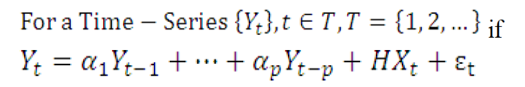
Where, Yt is the column vector of k-dimensional endogenous variables, Xt is the column vector of d-dimensional exogenous variables, p is the lag order, and T is the number of samples. The k×k - dimensional matrix Ф1…. Фp and k×d - dimensional matrix H are the coefficient matrices to be estimated. ɛt is a k-dimensional perturbed column vector, independent of its own lag values and independent of the variables on the right side of the equation. The ɛt is independently and identically distributed at different times, and if it follows a normal distribution, this equation is a p -order vector autoregression model. The stochastic process satisfying this model is a P-order vector autoregression process, denoted as VAR(p). This is the standard VAR model, or simplified model.

Long-term and short-term relationships are two important relationships between data series. If two sequences have a Co-integration, then there is a long-term relationship between them, and any temporary short-term deviation will be corrected. Let us illustrate the ECM by taking variables x1t and x2t as examples. It is assumed that there is Co-integration between these two variables.

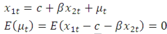
Where x1t and x2t are all first-order integral variable, that is I(1). If the residual series et obtained after regression is stable, there exists a long-term equilibrium relationship between x1t and x2t. However, in the short term, if the non-equilibrium state (μt ≠ 0) curs at stage t-1, x1t and x2t must be corrected or adjusted to try to return to the equilibrium state. This adjustment process is the Error Correction Process, and if modeled, it is called the Error Correction Model:

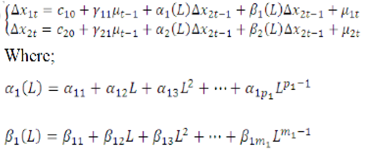
In a similar way, α2(L) and β2(L) can be defined, and the number of lags can be selected by information criteria. Among them, γ11 and γ21 are the modified velocity coefficients. Please refer to the relevant references (Meidinger, 1980; Box et al., 2015; Hamilton, 2020). We will discuss in detail the points worth attention in the application of the models in the next section.

RESULTS AND DISCUSSION

Long-term price relation analysis (based on the ECM model)

The results of the ADF test are shown in Table I. We found that BP, IBP, and ISP could not reject the null hypothesis of “unit root,” that is, they are all non-stationary sequences at the level of 5%. We test each variable again after the first-order difference, and then all the variables become stationary time series, that is, the null hypothesis can be rejected at the level of 1%, and all sequences are first-order integral variables I (1).

 

Table I. Results of ADF test.

variable	Prob.**	Test type (C, T, K)	T statistics	Results
LNBP	0.9811	(0,0,2)	1.7611	non-stationary series
LNISP	0.3075	(1,0,1)	-1.9529	non-stationary series
LNIBP	0.0639	(1,0,2)	-2.7768	non-stationary series
D(LNBP)	0.0000	(1,0,0)	-6.0958	stationary series
D(LNISP)	0.0000	(0,0,0)	-8.0290	stationary series
D(LNIBP)	0.0000	(0,0,4)	-8.1098	stationary series

 

Note: (1) LNBP is the logarithm of BP, and DLNBP is the first difference of LNBP. Other series are obtained in the same way. (2) C, T and K is intercept term, trend term and lag order, respectively.

 

Johansen cointegration test

The Johansen test method is based on the VAR model, and can test the co-integration relationship of multiple variables, which was suitable for this study (Aguirre and Aguirre, 2000; Box et al., 2015). Every series contains 159 observations, so the preferred maximum lag order is 10. The optimal lag order was determined to be 10 according to the five indicators: LR (Likelihood ratio) statistics, FPE (Final Prediction Error) final prediction error, AIC (An Information Criterion) information criterion, SC (Schwarz criterion) information criterion, and HQ (Heckscher-Ohlin) information criterion. Through Johansen co-integration model analysis, the test form is the trend determination test (trend assumption: linear deterministic trend). The test results are listed in Table II.

Both the trace test results and the maximum eigenvalue test results show that the null hypothesis that “there is no co-integration relationship among ISP, IBP and BP” can be rejected at a significance level of 5%, but the null hypothesis that “there is at most one co-integration relationship” cannot be rejected. Therefore, it can be judged that there is a significant long-term stable equilibrium among IBP, ISP, and BP; i.e., in the end, when ISP and IBP change, BP is affected. According to the co-integration relationship, the co-integration equation can be written to express the long-term co-integration relationship between the three sequences, as shown below:

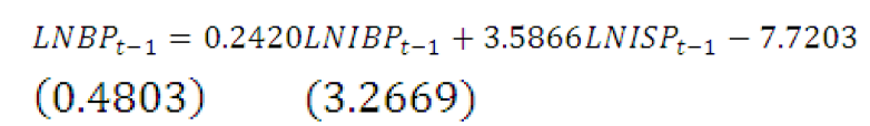
First, there is a significant positive correlation between BP and ISP, and IBP in the end. The co-integration equation shows that if ISP and IBP change by 1%, BP will change by 3.59% and 0.24%, respectively, in the same direction. Second, ISP has a very strong influence on the long-term fluctuation of BP, while IBP has a weak influence on the long-term fluctuation of BP. According to the complete market theory, the price change at the end of the industrial chain will be transmitted to the front of the industrial chain, resulting in the disturbance of different proportions of prices in the front (Marsh, 1994; Dong et al., 2014). In the beef industry chain, the impact of ISP on BP reached 3.59%, indicating that the long-term ISP has a very strong impact on BP. However, the transmission ratio of IBP to BP is 0.24%, indicating that BP in China is not very sensitive to IBP in the end.

 

Table II. Results of Johansen Cointegration test.

Hypothesized No. of CE(s)	Eigen value	Trace statistic	Prob.**	Max eigen statistic	Prob.**
None *	0.1348	31.1746	0.0345*	21.5759	0.0433*
At most 1	0.0526	9.5987	0.3129	8.0454	0.3741
At most 2	0.0104	1.5534	0.2126	1.5534	0.2126

 

* denotes rejection of the hypothesis at the 0.05 level; **MacKinnon-Haug-Michelis (1999) p-values.

 

 

Error correction model estimation

The Johnson cointegration test shows that there is a long-term equilibrium relationship between BP and ISP and IBP, but the prices are not synchronized in the short term. Therefore, the influence of short-term price fluctuations on each other should be analyzed, and the ECM model should be established to adjust for short-term fluctuations and make them conform to the long-term trend (LeSage, 1990). Here, the maximum likelihood estimation method is used for regression analysis of the model, and the estimated values of the parameters obtained are shown in Table III.

 

Table III. Results of ECM estimate.

Error correction: D(LNBP)			Series	Coefficient	T-statistics	Series	Coefficient	T-statistics
Series	Coefficient	T-statistics
			CointEq1	0.0004	-0.0013	C	0.0018	-0.0010
D(LNBPt-1)	0.5549	-0.0882	D(LNIBPt-1)	-0.0123	-0.0034	D(LNISPt-1)	0.0154	-0.0186
D(LNBPt-2)	0.1215	-0.1001	D(LNIBPt-2)	-0.0151	-0.0041	D(LNISPt-2)	0.0271	-0.0190
D(LNBPt-3)	0.1086	-0.1000	D(LNIBPt-3)	-0.0115	-0.0046	D(LNISPt-3)	0.0194	-0.0190
D(LNBPt-4)	-0.0058	-0.0931	D(LNIBPt-4)	-0.0017	-0.0045	D(LNISPt-4)	-0.0201	-0.0189
D(LNBPt-5)	-0.0549	-0.0930	D(LNIBPt-5)	0.0018	-0.0041	D(LNISPt-5)	-0.0366	-0.0190
D(LNBPt-6)	0.1098	-0.0943	D(LNIBPt-6)	-0.0003	-0.0042	D(LNISPt-6)	0.0412	-0.0193
D(LNBPt-7)	-0.0478	-0.0923	D(LNIBPt-7)	-0.0102	-0.0042	D(LNISPt-7)	-0.0116	-0.0191
D(LNBPt-8)	0.1216	-0.0874	D(LNIBPt-8)	-0.0059	-0.0040	D(LNISPt-8)	0.0077	-0.0192
D(LNBPt-9)	-0.1433	-0.0716	D(LNIBPt-9)	-0.0065	-0.0032	D(LNISPt-9)	0.0080	-0.0185

 

 

The results show that most coefficients of the ECM model are significant at the 5% level. When BP deviates from the long-term trend in the short term, the short-term fluctuation can be adjusted to the long-term equilibrium state through error correction. The error correction coefficient of the comprehensive model was 0.04. When BP fluctuation exceeds 1% of IBP or ISP, in the next period, BP would drop by 0.04% on average, and the overall adjustment speed is relatively slow. The error correction coefficient (-1≤β≤0) indicates the speed of adjustment to equilibrium. The closer the error correction coefficient is to 0, the slower the correction speed will be, and vice versa (Piesse et al., 2011).

Short-term price relation analysis (based on VAR model)

The results of the ECM model show that there is a long-term equilibrium relationship among the three series, and the long-term trend can be achieved under the action of a short-term adjustment mechanism (LeSage, 1990; Enders, 2014). However, it does not reflect the relationship between BP and the reaction cycle and adjustment time lag of IBP and ISP.

 

Therefore, the VAR model is applied to analyze the influence of independent variable changes on current and future dependent variables through the dynamic relationship between variables. Therefore, it can be used to analyze the relationship between BP and ISP and IBP. The VAR model adopted can be displayed as;

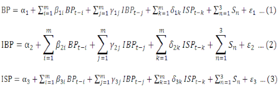
Where t stands for time; α is the constant term of each equation; β is the coefficient of the lag term of BP in the three equations; γ is the coefficient of IBP lag term in each equation; δ is the coefficient of the ISP lag term in each equation, S is three seasonal dummy variables, ε is the error term for each equation, and the expected value of the error term is 0.

Unit root test

The previous test showed that the first-order difference of all sequence variables reached a plateau at a credibility level of 5%. To further eliminate the seasonal influence, three dummy variables are added to the three series in the VAR model (Box et al., 2015). In the new VAR model, the lag order is determined by the same method as above, and the optimal lag order is 6. The unit root test results show that all roots are within the unit circle, indicating that the VAR (6) model is stable and can be analyzed further. The unit root test results are shown in Figure 4.

 

Granger causality

In order to determine the relationship between BP and ISP, IBP, a Granger causality test should be conducted. The lag order of Granger causality test was selected according to the principle of AIC and SC. The results are shown in Table IV.

According to the test results, the null hypothesis “IBP is not the granger cause of BP” was rejected at the 1% confidence level, the null hypothesis “BP are not the granger cause of IBP” was rejected at the 5% confidence level; therefore, the IBP and BP are granger causality. The null hypothesis “ISP is not the granger cause of BP” was rejected at the 1% confidence level and passed the test, but “BP is not the granger cause of ISP” was not rejected at the 5% confidence level. This shows that ISP is the main reason for BP, while BP is not the main reason for ISP. When the ISP and IBP are the explanatory variables and BP is an explanatory variable, the model rejected the null hypothesis (“ISP, IBP are not granger cause of BP”) at the 1% confidence level overall. Therefore, the VAR model in the form of formula (1) can be used to analyze the changing relationship between ISP, IBP, and BP, and the VAR model can continue to be used for impulse response analysis and variance decomposition (Hamilton, 2020).

 

Table IV. Results of granger causality.

Null Hypothesis	Chi-sq	Df	Prob.
IBP is not the granger cause of BP	30.2733	6	0.0000
ISP is not the granger cause of BP	18.9314	6	0.0043
ISP, IBP are not granger cause of BP	48.9165	12	0.0000
BP are not the granger cause of IBP	15.6534	6	0.0157
ISP is not the granger cause of IBP	5.5349	6	0.4772
BP and ISP are not granger cause of IBP	19.3711	12	0.0800
BP are not the granger cause of ISP	4.1301	6	0.6591
IBP is not the granger cause of ISP	8.6963	6	0.1914
BP and ISP are not granger cause of IBP	12.9684	12	0.3713

 

Impulse response analysis

The regression results of the VAR model were used for impulse response and variance decomposition analysis to help understand the impact of the changes of endogenous variables in the model on other variables and themselves, to analyze the dynamic changes among variables (Box et al., 2015). We applied a Cholesky One S.D. Innovations impulse to the system to obtain the impulse response function, which reflects the dynamic relationship of 20 cycles.

According to Figure 5, BP showed a time-delay facing a standard impact on IBP and ISP, both of which started from the second phase. BP showed a positive reaction to the impact of ISP, but this reaction was slow and gentle. It reached the first peak of 0.0021 in the fourth stage, reached the second peak in the seventh stage, and then began to converge. It converged to 0 around the 17th stage, and then the influence gradually disappeared. The reaction of BP to IBP was negative at first and then showed an alternate state. The peak value was 0.0026 in the sixth phase, and gradually converged to 0 after the 14th phase, and finally the influence gradually disappeared.

The result of the impulse response shows that the impact of IBP on BP is negative, which indicates that the increase in beef price change rate does not translate into the rational growth of domestic beef production (Goodwin and Holt, 1999; Darbandi and Saghaian, 2016; Hamilton, 2020). Under the stimulation of the rising IBP, all the raisers will increase the domestic beef cattle supply. First, by shortening the breeding time by 1-2 months, beef cattle will be brought out of the market. Second, the beef cattle stock will increase, resulting in the short-term periodic fluctuation of domestic beef supply and the periodic fluctuation of beef price. It is reflected in the pulse response diagram that the price decreases around the second to the third month and then pulls back to the vicinity of 0 in the fourth month. However, due to the overlapping effects of early acceleration and a shortened breeding cycle, the domestic beef cattle production volume was lowest in the sixth month, market supply was limited, and the price rose with the largest amplitude. From the 8th to the 10th month, the newly added beef cattle and the increased stocks after the shortened breeding cycle began to be put out of stock at the same time, and the domestic beef market price dropped again. The influence of this price cycle fluctuation lasted for 2 cycles until the 14th period when the cobweb fluctuation effect gradually disappeared.

Variance decompositions

Variance decomposition is the degree to which the impact of each variable in the analysis model affects the endogenous variables, and is used to describe the importance of the impact in the dynamic changes of ISP and IBP (Box et al., 2015). In this study, the Cholesky decomposition method was chosen. The number of decomposition phases is 20, and the decomposition results are shown in Table V.

As can be seen from Table V, BP was not affected by ISP and IBP in the first phase, but gradually decreased to 84% over time due to its own factors, and gradually increased under the influence of IBP and ISP. The IBP increased from the second phase onwards, reaching 9.81% in the fifth phase, and was subsequently maintained between 8% and 9%. The contribution rate of ISP to BP showed an upwards trend, rising from the second period and reaching the maximum fluctuation of 8.38% in the sixth period, and then maintaining a fluctuation between 7% and 8%. The impact of ISP on BP is relatively small compared to the impact of IBP.

 

Table V. Results of variance decomposition.

Period	S.E.	DLNBP	DLNIBP	DLNISP	Period	S.E.	DLNBP	DLNIBP	DLNISP
1	0.0071	100.000	0.0000	0.0000	11	0.0124	84.3037	7.5284	8.1679
2	0.0082	94.4732	2.9077	2.6191	12	0.0126	84.5400	7.4766	7.9834
3	0.0093	88.9084	4.3857	6.7059	13	0.0128	84.5798	7.5241	7.8961
4	0.0102	86.5131	3.6851	9.8019	14	0.0129	84.6783	7.3790	7.9427
5	0.0107	86.6270	3.5660	9.8071	15	0.0131	84.6323	7.2628	8.1050
6	0.0113	82.7827	8.3773	8.8400	16	0.0131	84.6866	7.1987	8.1147
7	0.0118	83.4680	7.7354	8.7966	17	0.0132	84.7582	7.1659	8.0759
8	0.0121	83.7898	7.6060	8.6042	18	0.0132	84.8509	7.1160	8.0332
9	0.0123	83.9358	7.6804	8.3838	19	0.0133	84.9405	7.0618	7.9977
10	0.0123	84.0593	7.6463	8.2944	20	0.0133	85.0160	7.0152	7.9688

 

Summary

The results of the empirical analysis verified that changes in IBP and ISP would lead to fluctuations in BP and affect beef demand. There is a long-term equilibrium relationship between ISP, IBP, and BP. Furthermore, there is a dynamic pass-through relationship between import price and domestic price, which can adjust short-term fluctuations to long-term trends through error correction (Liu and Yang, 2015; Hamilton, 2020). Although there is a cointegration relationship among the prices of the three series in the long term, its error correction term coefficient tends to 0. This shows that when ISP is impacted, BP would deviate from equilibrium, the speed of returning to equilibrium is slow, which also shows that the frequent disturbance of import price is likely to cause chaos in the domestic beef industry’s price system in the short term (Dong et al., 2014). In general, the impact of SBP or ISP on BP is low in the long term.

In summary, BP shows three characteristics when facing the impact of ISP and IBP. First, there is a delay in the reaction. When facing the impact, BP showed a time lag of 1 month before the reaction. Second, the fluctuation range is small. BP shows the largest response to the impact of IBP, but the maximum amplitude is only 0.0026, while the maximum response amplitude to the impact of ISP is only 0.0021. Both series affected BP for more than one year. The effect of IBP peaked in the 6th month and then showed convergence, but gradually disappeared after the 14th month. The effect of ISP showed convergence after the 4th month, but it did not converge to 0 until the 17th month.

The impulse response reflects the existing problems in domestic beef cattle breeding, such as the lack of modern management mode, the small scale of breeding, and the lack of large-scale farms (Dong et al., 2014; Xue and Yan, 2019). The current situation in which the beef cattle supply is dominated by small farmers has affected the development of China’s beef cattle industry. Small farmers show collective irrationality in the face of short-term interests, such as accelerating the listing and massively increasing the inventory, which will also drive the increase in the price of means of production and production costs. As a result, the short-term beef supply is not stable and the market fluctuates strongly, without bringing substantial benefits to farmers. In contrast, the negative effect held dominant position, and expression was an increase in production, not an increase in effect (Dong et al., 2014).

The domestic beef market is becoming increasingly internationalized (Diakosavvas, 1995), which is not only influenced by the price of imported beef, but also by fluctuations in international soybean prices. The production mode dominated by small farmers lacks the concept of long-term interests, market management thoughts, and modern management concepts, and cannot meet the requirements of China’s current supply side structural reform (Dong et al., 2014; Xue and Yan, 2019), which has become an important factor restricting the development of the domestic beef cattle industry. Second, the independence of the basic means of production will affect many domestic industries, or even national security and the safety of people’s lives. China’s soybean market is heavily dependent on foreign countries. The international soybean market will cause fluctuations in a wide range of domestic industries, such as the breeding and processing industries of beef cattle, sheep, swine, and poultry, which will affect the food structure of residents and affect national security and people’s living standards.

The empirical analysis of beef cattle industry has proved that the international soybean price will inevitably bring about the fluctuation of domestic beef price in the long run. China is heavily dependent on imports of soybeans, and the supply and demand of the international market affect the production cost of animal husbandry, thus affecting domestic animal husbandry products and market. The international market seriously affects the independent production of domestic animal husbandry and the independent operation of domestic animal product market (Hall, 2020).

China is the country with the largest population in the world, and the domestic supply of livestock products is insufficient, so import is an important way to meet the domestic demand. Poultry and pork are the main imported meat, while the import of beef and mutton is increasing gradually in recent years (Duan et al., 2019). In this research, the relationship between imported beef and domestic beef prices has reflected that international beef will affect the domestic beef market, so other animal products market is more difficult to avoid. In a word, when the Means of Agricultural Production Market and the livestock product markets are both impacted by the international market, it is difficult for domestic animal husbandry to develop independently.

CONCLUSION

The stable development of a country’s industry and the win–win result of openness may be two contradictory concepts. Therefore, a country’s openness to the outside world should be considered in the same manner as the issue of national security. To ensure the smooth operation of the domestic market, multiple measures should be taken. We found that for an open country, whether at the input end or the output end, the degree of dependence on the international market is an important factor determining industrial independence. That is, if the Means of Production Market and the product markets are both impacted by foreign countries, it is difficult for domestic industry to develop independently. Nor is China a complete winner in international trade. In fact, China has sacrificed many aspects in international trade, such as the independent development of industries. Agriculture is the basic industry and the foundation of all other industries such as manufacturing industry and service industry. The independent development of animal husbandry is related to the living standard of the residents and the security of the country. It should be taken seriously. First, the open country should diversify its import markets to reduce monopoly risks. This will help prevent international agricultural prices from fluctuating adversely on domestic prices. It should expand domestic production, increase self-sufficiency, and reduce external dependence, especially for basic agricultural products, such as wheat, corn, soybeans, and other food crops. Second, the price warning mechanism is necessary. The open country should pay close attention to international market prices, promote the national reserve mechanism reform, and improve the ability to resist risks. Third, the most important factor is to actively cultivate new agricultural business entities, improve the quality of beef cattle industry operators, strengthen the research and development of marketing links and sales markets, improve the level of scientific management and scientific decision-making, support the construction of large-scale farms and breed improvement, and improve the output level and efficiency of agriculture.

ACKNOWLEDGMENTS

Authors acknowledge the support from Modern Agricultural Industrial Technique System of Hebei Province: Industrial Economic Position of Innovation Team Focusing on Beef Cattle (HBCT2018130301), Scientific Research Foundation for the Ph.D. (Hebei Agricultural University, No. YJ201841), and the China Scholarship Council (CSC NO. 201908130188).

Statement of conflict of interest

The authors have declared no conflict of interest.

REFERENCES

Aguirre, A. and Aguirre, L.A., 2000. Time series analysis of monthly beef cattle prices with nonlinear autoregressive models. Appl. Econ., 32: 265-275. https://doi.org/10.1080/000368400322697

Box, G.E., Jenkins, G.M., Reinsel, G.C. and Ljung, G.M., 2015. Time series analysis: Forecasting and control. John Wiley and Sons, Hoboken, New Jersey, USA.

Brester, G.W., 1996. Estimation of the US import demand elasticity for beef: The importance of disaggregation. Rev. Agri. Econ., pp. 31-42. https://doi.org/10.2307/1349664

Darbandi, E. and Saghaian, S., 2016. Vertical price transmission in the US beef markets with a focus on the great recession. J. Agribus., 34: 99-120.

Diakosavvas, D., 1995. How integrated are world beef markets? The case of Australian and US beef markets. Agric. Econ., 12: 37-53. https://doi.org/10.1016/0169-5150(94)00028-Z

Dong, L., Li, Q. and Cui, X., 2014. Analysis of beef price trend and its causes in China. Price Ther. Prcat., 1: 87-88-96.

Dong, X., Waldron, S. and Zhang, C.B.J., 2018. Price transmission in regional beef markets: Australia, China and Southeast Asia. Emirates J. Fd. Agric., pp. 99-106. https://doi.org/10.9755/ejfa.2018.v30.i2.1601

Duan, Y., Wang, A. and Ouyang, S., 2019. The present situation of livestock product trade of China and its international competitiveness measurement analysis. China Econ. Trade Herald., 23: 17-20. https://doi.org/10.35611/jkt.2019.23.3.20

Enders, W., 2014. Applied econometric time series. 4th ed, John Wiley and Sons, New York, Alabama, USA.

Goodwin, B.K. and Holt, M.T., 1999. Price transmission and asymmetric adjustment in the US beef sector. Am. J. agric. Econ., 81: 630-637. https://doi.org/10.2307/1244026

Hall, D., 2020. National food security through corporate globalization: Japanese strategies in the global grain trade since the 2007–8 food crisis. J.Peasant Stud., 47: 993-1029. https://doi.org/10.1080/03066150.2019.1615459

Hamilton, J.D., 2020. Time series analysis. Princeton University Press, Princeton, USA.

Han, Y., 2020. Global soybean market trend and selection and utilization of feed protein. Vet. Orient., 5: 5-6.

Hejazi, M., Marchant, M.A., Zhu, J. and Ning, X., 2019. The decline of U.S. export competitiveness in the Chinese meat import market. Agribusiness, 35: 114-126. https://doi.org/10.1002/agr.21588

Huang, P., Wang, J. and Meng, X., 2018. Rebalancing of economic globalization and the trade dispute between China and the United States Chin. Ind. Econ., 10: 156-174.

Jacks, D.S., O’Rourke, K.H. and Williamson, J.G., 2011. Commodity price volatility and world market integration since 1700. Rev. Econ. Stat., 93: 800-813. https://doi.org/10.1162/REST_a_00091

Jin, H.J., 2020. Driving factors behind consumers’ severe response to U.S. beef imports during the candlelight protest in South Korea. Agribusiness, https://doi.org/10.1002/agr.21671

LeSage, J.P., 1990. A comparison of the forecasting ability of ECM and VAR Models. Rev. Econ. Stud. Stat., pp. 664-671. https://doi.org/10.2307/2109607

Liu, X. and Yang, H., 2015. Analysis of correlative factors of beef price increase in China based on VAR model. China Price, 2: 58-60.

MARA, 2018. China animal husbandry and veterinary yearbook. China Agricultural Press, Beijing, China.

Marsh, J.M., 1994. Estimating intertemporal supply response in the fed beef market. Am. J. agric. Econ., 76: 444-453. https://doi.org/10.2307/1243656

Meidinger, E.E., 1980. Applied time series analysis for the social sciences. Sage Publications, Beverly Hills.

MOFCOM, 2020. Economic and trade agreement between the government of the People’s Republic of China and the government of the United States of America. http://www.mofcom.gov.cn/index.shtml. (accessed 2 Nov 2020).

NCNA, 2018. The Ministry of Commerce responded to the US proposal to impose tariffs on $200 billion of Chinese goods: it will take necessary countermeasures depending on the action taken by US. http://www.gov.cn/xinwen/2018-09/06/content_5319851.htm. (accessed 3 Nov 2020).

Piesse, J., Schimmelpfennig, D. and Thirtle, C., 2011. An error correction model of induced innovation in UK agriculture. Appl. Econ., 43: 4081-4094. https://doi.org/10.1080/00036841003800856

Rezitis, A.N. and Stavropoulos, K.S., 2010. Modeling beef supply response and price volatility under CAP reforms: The case of Greece. Fd. Policy, 35: 163-174. https://doi.org/10.1016/j.foodpol.2009.10.005

Savell, J.W., Cross, H.R., Francis, J.J., Wise, J.W., Hale, D.S., Wilkes, D.L. and Smith, G.C., 1989. National consumer retail beef study: Interaction of trim level, price and grade on consumer acceptance of beef steaks and roasts. J. Fd. Qual., 12: 251-274. https://doi.org/10.1111/j.1745-4557.1989.tb00328.x

Tang, L., 2017. Efficient feeding technology. Handbook. Tianjin Science and Technology Press, Tianjin, China.

Tian, L., Wang, J. and Zhang, Y., 2012. The dynamic change of beef market price in China and its correlation effect analysis. Issues agric. Econ., 33: 79-83.

Tian, W.M., 2017. Grains in China: Foodgrain, feedgrain and world trade. Routledge. https://doi.org/10.4324/9781351157087

Wang, W., 2007. Why does not correspond between China’s soybean trade status and international pricing power. Intertrade, 6: 9-13.

Xu, H., 2015. China and Australia have signed a free trade agreement, and tariffs on beef, dairy products and other goods will be reduced and reduced. China Fd., 13: 140.

Xue, Y.J. and Yan, J.L. 2019. Breeding efficiency of beef cattle in Chinese suitable areas. J. Anim. Pl. Sci., 29: 1413-1423.

Yoon, J. and Brown, S., 2016. Beef market integration and price transmission in the trans-pacific partnership (TPP) countries. No. 967-2016-75121. 2016.

Yu, J., Qiao, J. and Qiao, Y., 2005. Empirical analysis of the relationship between International trade and domestic market price of Chinese soybean. Issues Agric. Econ., 2015: 33-37.

Zhou, Y. and Wang, W., 2018. The analysis on market structure and demand elasticity of beef import in China. Price: Theory Pract., 3: 103-106.