Research Article

Supply Response Analysis of Wheat Growers in District Swabi, Khyber Pakhtunkhwa: Farm Level Analysis

Farhan, Shahid Ali* and Syed Attaullah Shah

Department of Agricultural and Applied Economics, The University of Agriculture, Peshawar, Khyber Pakhtunkhwa, Pakistan.

Received | December 09, 2018; Accepted |Januar29, 2019; Published | February 28, 2019

*Correspondence | Shahid Ali, Assistant Professor, Department of Agricultural and Applied Economics, The University of Agriculture, Peshawar, Pakistan; Email: drshahid@aup.edu.pk

Citation | Farhan, S. Ali and S.A. Shah. 2019. Supply response analysis of wheat growers in district Swabi, Khyber Pakhtunkhwa: farm level analysis. Sarhad Journal of Agriculture, 35(1): 274-283.

DOI | http://dx.doi.org/10.17582/journal.sja/2019/35.1.274.283

Keywords | Wheat output supply, Input demand, Elasticities, Translog profit function, Khyber Pakhtunkhwa-Pakistan

Introduction

Agriculture plays a vital role in Pakistan’s economy. It shares 18.90 percent to the Gross Domestic Product (GDP) and employs about 42.3 percent of the labour force. In rural areas of the country about 68 percent people are involved directly or indirectly in agriculture through production, processing, transportation and distribution of agricultural commodities. Being an important sector of the country’s economy, it provides raw materials to industries and also contributes to export earnings. It is further categorized to four subsectors such as crops, livestock, forestry and fisheries; each of which has a significant contribution to the economy (GoP, 2018).

Among the major cereal crops grown in Pakistan, wheat (Triticum aestivum) is a cereal grain used as a staple food worldwide. It belongs to family Poaceae of kingdom Plantae, first cultivated in Fertile Crescent’s regions about 9600 BCE ago. It is an important source of carbohydrates, proteins, nutrients, essential amino acids and dietary fibre. It provides energy of 1,368 kilo joules per 100 gram and is used as food in many ways such as bread, porridge, biscuits, pies, cakes, pastries and cookies etc. (Wikipedia, 2018).

Wheat can be grown twice in a year such as in spring and winter. The global wheat production was recorded as 749,460,077 tonnes within an area of 220,107,551 hectares and the global wheat yield was recorded as 3.40 tons per hectare (FAO, 2016). Among all the wheat grower countries in the world, China is the leading one followed by India, Russia, United States, Canada, France, and Ukraine. Pakistan is ranked as 8th with the total wheat production of 26,005,213 tonnes and the total cultivated area was 9,143,097. Wheat yield in Pakistan was recorded as 2.84 comparatively low than global wheat yield (FAO, 2016). This gap may be due to inefficiency of farmers or stochastic random effects such as floods, huge rainfall and climate change etc.

In Pakistan, Punjab is the leading wheat producer province followed by Sindh, Khyber Pakhtunkhwa and Baluchistan. The higher production in Punjab might be due to supply response of wheat crop in the province. Wheat production in Khyber Pakhtunkhwa can be improved by supporting wheat prices or by subsidizing the essential inputs required in production process.

In Khyber Pakhtunkhwa district Swat is the top producer of wheat with production of 111.3 tonnes followed by DI Khan, Mardan, Swabi, and Mansehra (Govt. of Khyber Pakhtunkhwa, 2016). In district Swabi wheat was grown on an area of 47.2 hectares and total production was recorded as 96.0 tonnes with an average yield of 2.03 which is low as compared to other districts Government of Khyber Pakhtunkhwa (GoPK, 2016). This low yield may probably be due to higher cost of production or lower prices of wheat output.

Utilization of input is deterred mostly by the lower prices of outputs but if the prices of output increase it tends to increase extra utilization of resources which brings to increase the profit. While prices of input increase it oppose the use of input and vice versa. (Goyal and Berg, 2004). In the presence of limited resources price policy and technical alterations play very important role for increasing agriculture production. Policy makers encounter a task to make appropriate policy for agriculture by which needed output would be achieved for this purpose it is necessary to know the responsiveness for inputs and output supply to the prices and technological alterations. These both input demand and supply of commodities are connected with each other. At the same time output supply and input demand is affected by changing the prices of input and output prices. Output supply is mostly decreased when cost of inputs are getting higher. Product prices increases by reduction in output supply (Thakare et al., 2012). Input demand and supply of output are directly connected, if any alteration occurs in prices of input and prices of products, output supply and input demand are affected. To make an efficient price policy and policy of food security so knowledge about the responsiveness of input demand and output supply to the prices of input and output and technology changes (Kumar et al., 2010). Analysis of input demand and output supply elasticities describes how much farmers are responsive to prices of output and inputs (Abrar et al., 2002).

Input demand and output supply elasticities have great importance for precise calculation of the responsiveness of wheat to change in input and output prices. Results of input demand and output supply elasticity provide a strong base in the advancement of policies which are applied which assist in production, efficiency and revenue circulation which is further helpful for the development of agriculture sector of the economy. No research work in the knowledge of this researcher has yet been conducted on supply response of wheat growers on farm level in district Swabi. This study is therefore an attempt to estimate input demand and output supply elasticities of wheat growers in district Swabi.

Due to different aspects this study has great importance. It helps the policy makers to know about the elasticities of different products whether they are elastic or inelastic and which will help them to recommend policies for wheat output and inputs involved in wheat production. The findings of this study are also important for researches to compare the results of this study with other findings.

Materials and Methods

This section deals with universe of the study, sample size and sampling technique, data and data sources, data collection and analytical techniques.

Universe of the study

This study was conducted in district Swabi of Khyber Pakhtunkhwa, Pakistan. Area of Swabi is 1543 square km. Swabi has productive soil and greatest capacity to grow wheat crop. Swabi is the 4th largest wheat producing district in Khyber Pakhtunkhwa.

Sample size and sampling technique

For selection of sampled wheat growers, a multi-stage random sampling technique was used. In 1st stage district Swabi was purposively selected being fourth largest wheat producing district of the province (Govt. of Khyber Pakhtunkhwa, 2017 and previous issues). District Swabi consists of tehsil Swabi and tehsil Razzar. In second stage tehsil Razzar was chosen randomly. In stage third, from a list of all major wheat producing villages, six villages namely Shewa, Permuli, Asota, Kalu Khan, Turlandi and Yar Hussain were selected randomly. In fourth stage a random sample of 160 was drawn by using Yamane formula (Yamane, 1967) as under:

 

Where;

n = sample size for wheat growers; N = total number of wheat growers; e = precision level.

160 wheat growers were randomly selected (Table 1) using technique of proportional allocation sampling by using Cochran (1977) as under:

 

Where;

ni = Sample size from ith village; n = Total sample size; Ni = Total wheat producers in ith village; N = population of wheat producers in all selected villages.

Data

In this study both primary and secondary data were used. Primary data from 160 sampled respondents were collected using a well-structured interview schedule. Face to face questions was asked from respondents on their fields and guest houses (locally known as Hujras). Though interview schedule is designed in English language but during data collection it was translated to Pashto language for convenience. Secondary data was taken from FAO, Pakistan Bureau of Statistics, Govt. of Khyber Pakhtunkhwa and Extension Department of District Swabi.

Data analysis

Cost and revenue of wheat crop: Following (Debertin, 2012; Varian, 1992) cost and revenue of wheat crop was determined by the formula as follows:

Net Revenue = Total Revenue –Total Cost …..(2)

Where;

Total Revenue = PYi × Yi ...... (3)

Total Cost =∑PXi x Xi …..(4)

Where;

PYi = Price per unit output(Rs/kg); Yi = wheat produced by ith wheat grower (Kg/acre); Xi = Inputs applied by ith wheat grower (unit); PXi = Prices of inputs (Rs unit-1).

Table 1: Sample size and sampling technique.

District	Tehsil	Villages	No. of wheat growers	Sample size
Swabi	Razzar	Shewa	90	28
		Permuli	70	22
		Asota	60	19
		Kalu Khan	80	25
		Turlandi	90	28
		Yar Hussain	120	38
		Total	510	160

Source: Govt. of Khyber Pakhtunkhwa, 2018.

Conceptual framework of the model: Envelope theorem: The envelope theorem states that the rate of change in S* (profit) with respect to a change in β, if all μi are allowed to adjust, is equal to the change in k with respect to the change in the parameter β when all μi are assumed to be constant.

Where;

S = the value need to be maximized; μi = variables; β = parameter; First order condition.

 

In terms of β the optimum value of μi = μ*i

 

Now i = 1, 2, 3,……..,n

Optimal values for Equation 3.5

The envelope theorem further states that the rate of change in S* with respect to a change in β, if all μi are allowed to adjust, is equal to the change in k with respect to the change in the parameter β when all μi are assumed to be constant.

 

First we take the partial derivative of Equation (8) with respect to β in order to prove Equation (9).

 

Hotelling’s lemma: Envelope theorem utilizes Hotelling’s Lemma for profit function. Total revenue is written for the firm which uses different number of inputs as r for the production of output t. total revenue Equation is:

 

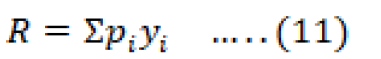
y1,……………….yt (Output)

Total cost of the inputs can be defined as:

 

For the firms expansion path shows output maximization combination in same case it defines the least cost combination of output. Maximization of revenue is represented by indirect function of revenue the equation depicts the optimal allocation of output.

 

Indirect cost function is represented as:

 

Difference between revenue and cost give us the indirect profit.

 

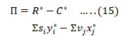
Alteration of input into output for profit maximizing is:

The production function enforced constrained for profit maximization the lagrangian multiplier is used.

 

First order condition.

i =1, 2, 3,…..t The optimum level yi is yi*

For factor side first order condition is:

i =1, 2, 3,…..n The optimum level of xi is xi*

Equation (16) is differentiated with pth price of the product.

 

Equation (18) and (19) are substituted into (20).

 

Now differentiate Equation (16) with pth price.

 

Substitute Equation (22) into (21).

 

Once again Equations (18) and (19) are substituted into (16) Indirect profit function can also be applied on factor side.

 

For product and input price equate both Equations (18) and (19).

Now with respect to pth input price differentiating Equation 3.17

 

Now substitute (26) into (25).

On factor demand side the hoteling lemma is applied change in indirect profit is with respect to change in factor demand price is equal to negative quantity of pth price.

The model: Following Sidhu and Baanante (1981), Farooq et al. (2001), Khan and Hussian (2007), Yaseen and Dronne (2011), Ullah et al. (2012) and Junaid et al. (2014) restricted normalized translog profit function was modelled as under:

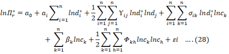
Πr*= Restricted profit, Πr is standardizing by price of output Pr ; di*= Input price di standardized by price of output Pr ; i=j=1, Labour wages; 2, Fertilizer; k = h = 1, Land Area; 2, Education; Ck= fixed input, k εi= Random error.

Measuring elasticities

Input demand elasticities: Own price elasticities of ith input demand (nii) was calculated as under:

Si is the share equation at the sample mean

Cross price elasticity of ith variable input demand in relation to jth variable input price (nij) was estimated as follows:

Demand elasticity of ith variable input with respect to output price (nir):

Elasticity of demand of ith variable input with respect to fixed mth factor (nim):

 

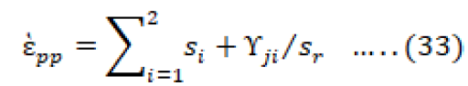
Output supply elasticity: Elasticity of wheat supply in response to own price of wheat ὲpp was estimated by Equation (33) as follows:

Elasticity of wheat supply in response to price of ith variable input ὲpi was estimated by Equation (34) as follows:

Output supply elasticity in relation to mth fixed factor ὲpm was calculated as under:

 

 

Profit elasticities: Elasticity of profit in response to price of ith variable input (ὲΠi) was computed by Equation (36) as below:

Elasticity of profit in relation to mth fixed factor (ὲΠm) was calculated by Equation (37) as under:

Diagnostic tests: Various diagnostic tests such as normality of residuals, heteroscedasticity and multicollinearity were performed for checking model adequacy.

Results and Discussion

This section presents cost of production, gross and net revenue, estimates of normalized restricted trans-log profit function, variable inputs’ demand equations, elasticities of profit, variable inputs’ demand and wheat output supply elasticities with respect to own price of wheat, wage rate, education, fertilizers price and area under wheat.

Cost of production

Table 2 describes cost of wheat production on per acre basis. Cost of production of wheat encompasses seed, ploughing, fertility input, irrigation, pesticides and weedicides, land rent, harvesting, threshing, bags and transportation cost. Land rent was 16700 Rs/Acre (37.87%) of the overall cost production followed by fertility inputs which is 4946.61 (11.21%), irrigation cost is 4727.44 (10.72%), threshing cost which is 4300 (9.75%), harvesting cost which is 3981.04 (9.02%), land preparation cost which is 3507.84 (7.95%), seed rate which is 2361.45 (5.33%), pesticide and weedicide cost which is 2112.15 (4.79%), transportation cost which is 951 (2.15%) and bags cost which is 510 (1.15%) cost of wheat production per acre. Total cost of production of wheat per acre was Rs. 44087.53 per acre.

Table 2: Cost of production (per acre).

Items Units Quantity Rate/unit Cost (Rs) %age Seed cost Kg 43.41 53.92 2351.45 5.33% Tractor cost Hrs 2.00 1088 2177.00   Labour cost Days 2.34 568.72 1330.84   Land preparation Rs     3507.84 7.95% Urea Kg 64.06 19.12 1224.82   Dap Kg 52.50 55.68 2919.00   Nitrophous Kg 27.64 7.98 220.80   Application cost(labour) Days 1.37 568.72 781.99   Fertility cost input Rs     4946.61 11.21% Irrigation cost of labour Days 2.00 568.72 1137.44   Irrigation* (electricity+ abiana) Days 2.00 1795.00 3590.00   Irrigation Rs     4727.44 10.72% Pesticides Bottles 1.00 707.50 707.50   Weedicides Bottles 1.00 835.92 835.93   Pesticides Weedicide Days 1.00 568.72 568.72   Pesticide and Weedicide Rs     2112.15 4.79% Harvesting cost (labour) Days 5.00 568.72 3981.04 9.02% Threshing cost Rs     4300.00 9.75% Land rent Rs     16700.00 37.87% Bags Rs 34.00 15.00 510.00 1.15% Transportation Rs     951.00 2.15% Total Cost Rs     44087.53 100%

Source: Authors’ estimates from survey data, 2017; * Irrigation cost: Electricity charges + Abiana

Gross and net revenue

Gross and net revenue of wheat crop is presented in Table 3. The average main product of quantity of wheat was recorded as 1746.25 kgs per acre, and Rs.29.93 is the average price of wheat per kgs, so the average gross revenue of the main product was calculated as Rs. 52,265 per acre, and average by-product quantity of wheat was recorded as 3492.50 kgs per acre, and 4.54 is the average price of by-product per kgs, the average gross revenue of by-product was calculated as 15864.21. Total gross revenue from production of wheat per acre was calculated as 68129.21 and net revenue was Rs. 24,041.68.

Table 3: Gross and net revenue (per acre).

Particulars	Quantity (kgs)	Price (Rs/kg)	Amount (Rs)
Main product	1746.25	29.93	52,265.00
By-product (Bhosa)	3492.50	4.54	15,864.21
Gross revenue			68,129.21
Total cost			44,087.53
Net revenue			24,041.68

Source: Authors’ estimates from survey data, 2017.

Estimated model

Descriptive statistics of the variables: Table 4 depicts mean, standard deviation, minimum and maximum values of the variables used in the estimation of restricted normalized translog profit function and input demand equations. On average, restricted profit of wheat growers was Rs. 34,377, with the standard deviation, minimum and maximum of 3,856, 25,650 and 45,996, respectively. Average mean value of fertilizer price was Rs. 55.68 per kg with standard deviation of 2.429 ranging from 54 to 70, respectively. Mean wages of labor was Rs 568.12, with the standard deviation of 67.639 ranging from 400 and 700. Average land (area) cultivated under wheat was 3.411 acres with standard deviation 1.422 ranging from, 1.25 and 8. Mean education level of the wheat growers was 9.675, with standard deviation, maximum and minimum of 2.136, 6 and 14 respectively.

Diagnostic tests: Histogram of residuals was drawn to check normality of error term. Histogram revealed that the distribution of the error term was normal. Thus, the normality assumption was accepted (Supplementary Figure 1). The problem of heteroscedasticity was detected in the estimated model. Heteroscedasticity was corrected by giving the command “robust” STATA 12 software. The results of this test are given as under:

Breusch-Pagan/Cook-Weisberg test for heteroskedasticity

Ho: Constant variance

Variables: fitted values of lnprofit

chi2(1) = 0.08

Prob>chi2 = 0.7718

VIF results revealed that this approximation was suffered from multicollinearity problem (Supplementary Table 1). Remedial measure of collinearity is that according to Gujarati and Porter (2009) do nothing because there will always occur relation between variables especially socioeconomic variables and as variables are BLUE, it would not affect the results. Inclusion of square and interaction terms of explanatory variables in this model is requirement of the functional form therefore these cannot be omitted.

Table 4: Descriptive statistics of the variables.

Variable	Unit	Mean	Std. Dev.	Min	Max
Restricted profit	Rs/acre	34,377	3,856	25,650	45,996
Fertilizer price	Rs/kg	55.68	2.429	54.00	70
Wage of labor	Rs/day	568.125	67.639	400	700
Land (Area under wheat)	Acres	3.411	1.422	1.25	8
Education	Years	9.675	2.136	6	14

Source: Authors’ estimates from survey data, 2018.

Table 5: Estimates of restricted normalized translog profit function and share equations.

	Intercept	lnPL	lnPF	lnC1	lnC2
Profit Function	11.395	-1.313	-1.99	3.621	2.89
	(0.26)	(-2.38)	(-3.43)	(1.95)	(0.80)
	(43.48)	(0.55)	(0.32)	(1.85)	(3.61)
Share equation of labor	-1.313	0.003	0.532	0.350	-0.624
	(-2.38)	(0.00)	(0.65)	(1.36)	(-1.28)
	(0.55)	(0.84)	(0.81)	(0.25)	(0.48)
Share equation of fertilizer	-1.099	0.532	-0.30	0.102	0.316
	(-3.43)	(0.65)	(-0.40)	(0.44)	(1.05)
	(0.32)	(0.81)	(0.75)	(0.23)	(0.30)
	(lnPL)2/2	(lnPF) 2/2	lnPLlnPF	lnPLlnC1	lnPLlnC2
	-0.003	-0.30	0.532	0.350	-0.624
	(-0.00)	(-0.40)	(0.65)	(1.36)	(-1.28)
	(0.84)	(0.75)	(0.81)	(0.25)	(0.48)
	lnPFlnC1	lnPFlnC2	lnC1lnC2	(lnC1) 2/2	(lnC2) 2/2
	0.102	0.316	0.403	0.033	-0.222
	(0.44)	(1.05)	(3.33)	(0.72)	(-1.12)
	(0.23)	(0.30)	(0.12)	(0.04)	(0.19)

Standard errors and t-ratios are in parenthesis; R2: 0.29; 0: Adj; R2: 0.2706; F: 4.23; Source: Authors’ estimates from survey data, 2018.

Estimates of restricted normalized translog profit function: Table 5 presents estimated parameters of the restricted normalized translog profit function and input demand equations. The parameter of the estimated equation is used to find out the input demand and output supply elasticities regarding wheat price, labour wages, fertilizer price, land area in acre and education. R2 revealed that regressors explained 29% variations in dependent variable. Calculated F statistic (4.23) confirms that the estimated model was good fit. This estimated model was also utilised for derivation of share equations of labor and fertilizer.

Derived elasticities: Table 6 portrays estimated output supply and input demand elasticities in response to wheat price, wage rate, fertilizer price, land (area under wheat crop) and education of farmers. Output supply and input demand elasticities were derived from estimated model of restricted normalized trans log profit and factor demand equations. All the signs of these results are consistent with the economic theory and discussed as under.

Table 6: Derived elasticities.

	Output price	Wage Price	Fertilizer Price	Land	Education
Output	1.984	-0.349	-1.817	6.082	0.588
Labor	6.131	-1.177	-4.972	3.583	2.964
Fertilizer	3.112	-0.485	-2.443	4.025	4.528
Profit	2.786	0.159	1.627	7.061	0.453

Source: Authors’ estimates derived from estimated models and share equations.

Output elasticities: Response of output supply to the price of wheat was estimated to be 1.984 (elastic); this means that 1% increase in price of wheat increases wheat output by 1.984%. It can be inferred from these estimates that increase in wheat price would encourage farmers to produce more wheat in future. Output supply in response to wage rate was - 0.349 (inelastic); implies that 1% rise in wage rate decreases output supply by 0.349%. Decrease in wheat output due to increase in wage rate was not substantial. Output elasticity in response to fertilizer price was – 1.817 (elastic). This means that increase in fertilizer price has negative effect on output and a percent increase in fertilizer price decreases output supply by 1.817 percent. Output supply in relation to land was 6.082 (elastic), this mean that a percent increase in area under wheat crop raises supply of wheat by 6.082%. Relationship between farm size and productivity is quite controversial. According to (Kiani, 2008) and few other researchers the farm size has negative relationship with production while according to Griffin (1976) farm size and output has positive relationship.

Education has positive relation with the output supply but inelastic (0.588). This implies that 1% increase in education increases output supply by 0.588%. These results are in conformity with the findings of Ullah et al. (2012) and Junaid et al. (2014).

Labor demand elasticities: Labour demand in relation to output price was estimated to be 6.131 (elastic). A percent rise in wheat price would raise the labour demand by 6.131%. The labour demand in relation to wage rate and fertilizer price was -1.177 and -4.972, respectively. This implies that a percent rise in wage rate and fertilizer price decreases demand for labour by 1.177% and 4.972 %, respectively. Labour demand in relation to land and education were positive and elastic. This means that one percent increase in land and education increases demand for labour by 3.583% and 2.964%, respectively.

Fertilizer demand elasticities: Elasticity of fertilizer demand in relation to wheat price was 3.112 (elastic). This implies that a 1% rise in wheat price increases demand for fertilizer by 3.112%. Wage rate has negative and inelastic effect on fertilizer demand. A percent rise in wage rate decreases demand for fertilizer 0.485%. Estimated own price elasticity for fertilizer demand was -2.443 (elastic); this means that 1% rise in fertilizer price decreases demand for fertilizer by 2.443%. Demand for fertilizer in response to land and education were 4.025 (elastic) and 4.528 (elastic), respectively. This implies that 1% increase in land and education increases demand for fertilizer by 4.025 and 4.528 percent, respectively. These results are in conformity with findings of Chaudhary et al. (1998).

Profit elasticities: Profit elasticities of wheat as a result of wheat price, fertilizer price and land were 2.786, 1.627 and 7.061, respectively. This infers that profit response to all these factors were positive and elastic. 1% increase in wheat price, fertilizer price and land increases profit of farmers by 2.786%, 1.627% and 7.061% percent, respectively. Response of profit due to wage rate and education were found be 0.159 and 0.453, respectively. This means that profit response to wage rate and education were positive but inelastic suggesting that 1% increase in wage rate and education increases profit by 0.159% and 0.453%, respectively.

Conclusions and Recommendations

This study estimated output supply and input demand elasticities of wheat in district Swabi of Khyber Pakhtunkhwa, Pakistan. For this purpose, 160 wheat growers were selected through multi-stage stratified random sampling technique. Primary data was collected through well design interview schedule. Normalized restricted translog profit function was first approximated for further estimation of output supply and input demand elasticities. Response of output supply to the price of wheat and land was positive and elastic. Output supply in response to wage rate was negative and inelastic. Output elasticity in response to fertilizer price was negative and elastic. Education has positive relation with the output supply but inelastic. Labor demand in response to output price, land and education was positive and elastic. Labor demand in relation to wage rate and fertilizer price was negative and elastic. Elasticity of fertilizer demand in relation to wheat price, land and education was positive and elastic. Wage rate has negative and inelastic effect on fertilizer demand. Estimated own price elasticity for fertilizer demand was negative and elastic. Profit elasticities of wheat as a result of wheat price, fertilizer price and land were positive and elastic. Response of profit to wage rate and education was positive but inelastic. In summary it can be concluded that wheat farmers are highly responsive to wheat own price in terms of output supply which in turn increases profit of farmers manifolds. Demand for fertilizer and labor increases with the decrease in their prices, thereby increasing the application of these inputs in the production of wheat.

As response of output supply of wheat and profit from wheat crop is price elastic therefore, government needs to set and declare increased procurement price of wheat prior to sowing season. This in response will lead to more supply, employment and profit. As with the decrease in price of fertilizer, demand for it increases therefore, wheat growers need to be facilitated with subsidized prices of fertilizer to encourage its application that will raise output and profit of wheat growers. As education positively affect output supply and profit of wheat therefore, trainings of wheat growers for optimal application of inputs for wheat crops be arranged at regular intervals by concerned departments for efficient utilization of resources and increased output.

Author’s Contribution

Farhan: Carried out this study and wrote first draft of the manuscript, reviewed literature and constructed methodology, collected and analyzed data.

Shahid Ali: Developed main idea of this study in collaboration with Farhan and Syed Attaullah Shah, wrote abstract, conclusion and recommendations. supervised overall write up of this paper.

Syed Attaullah Shah: Provided guidance in analysis, interpretation of results and comparison of findings with other studies.

Supplementary Material

There is supplementry material associated with this article. Access the material online at http://dx.doi.org/10.17582/journal.sja/2019/35.1.274.283

References

Abrar, S., O. Morrissey and T. Rayner. 2002. Supply response of peasant farmers in Ethiopia. Centre Res. Econ. Dev. Int. Trade, Univ. Nottingham.

Chaudhary, M.A., M.A. Khan and K.H. Naqvi. 1998. Estimates of farm output supply and input demand elasticities: Pak. Dev. Rev. 37(4): 1031-1050. https://doi.org/10.30541/v37i4IIpp.1031-1050

Cochran, W.G. 1977. Sampling techniques, 3rd Edition. John Wiley and sons, New York. pp. 37–45.

Debertin, D.L. 2012. Agriculture production economics, 2nd Edition. Macmillan publishing company, New York.

Farooq, U., T. Young, N. Russell and M. Iqbal. 2001. The supply response of basmati rice growers in Punjab, Pakistan: J. Int. Dev. 13(2): 227-237. https://doi.org/10.1002/jid.728

Food and Agricultural Organization (FAO). 2016. Year wise world wheat statistics, http://www.faostat.fao.org.

GoP. 2014. Economics survey of Pakistan, 2015-16. Economic advisory wing, finance division, Islamabad, Pakistan

GoP. 2016. Economics survey of Pakistan, 2015-16. Economic advisory wing, finance division, Islamabad, Pakistan.

GoP. 2018. Economics Survey of Pakistan, 2017-18. Economic advisory Wing, Finance Division, Islamabad, Pakistan.

Government of Khyber Pakhtunkhwa. 2016. Development Statistics of Khyber Pakhtunkhwa. Bureau of Statistics, Planning and Development Department of Khyber Pakhtunkhwa. www.kpbos.gov.pk

Government of Khyber Pakhtunkhwa, 2017. Development Statistics of Khyber Pakhtunkhwa. Bureau of Statistics, Planning and Development Department of Khyber Pakhtunkhwa. www.kpbos.gov.pk

Goyal, S.K. and E. Berg. 2004. Estimating input demand and output supply on wheat farms in Haryana State of India. J. Gokhale Inst. Polit. Econ. 46(3-4): 361-372. Am. Agric. Econ. 237-246.

Griffin, J.M. and P. Gregory. 1976. An intercountry translog model of energy substitution responses. Am. Econ. Rev. 66(4): 845–857.

Gujarati, D.N. and D.C. Porter. 2009. Basic Econometrics, 5th Edition. McGraw Inc., New York.

Junaid, S., S. Ali, S. Ali, A. Jan and S.A. Shah. 2014. Supply response analysis of rice in Pakistan: Normalized restricted translog profit function approach. Int. J. Innov. Appl. Stud. 7(3): 826-831. http://www.ijias.issr-journals.org/

Khan, R.A. and S.M.A. Hussian. 2007. Farm supply response to price: A case study of sugarcane in Pakistan. J. Independent Stud. Res. (JISR), 5(2): 41-44.

Kiani, A.K. 2008. An empirical analysis TFP gains in agriculture crop sector of Punjab: A multi criteria approach. Eu. J. Sci. Res. 24(3): 339-347.

Kumar, P., P. Shinoja, S.S. Rajua, A. Kumara, K.M. Richb and S. Msangic. 2010. Factor demand, output supply elasticities and supply projections for major crops of India: Agric. Econ. Res. Rev. 23: 1-14.

Olwande, J.O. 2008. Maize supply response in Kenya: A farm-level analysis. http://ageconsearch.umn.edu.

Sidhu, S.S., C.A. Baanante. 1981. Estimating farm level input demand and wheat supply in the Indian Punjab using a translog profit function. Ame. J. Agric. Econ. 63(2,): 237–246. https://doi.org/10.2307/1239559

Thakare, S.S., N.V. Shende and K.J. Shinde. 2012. Mathematical modeling for demand and supply estimation for cotton in Maharashtra. Int. J. Sci. Res. Publ. 2(3): 1-5.

Ullah, R., S. Ali, Q.S. Safi, J. Shah and K.H. Khan. 2012. Supply response analysis of wheat growers in district Peshawar, Pakistan. Int. J. Latest Trends Agric. Food Sci. 2(1): 33-38.

Wikipedia. 2018. https://en.wikipedia.org/wiki/Wheat Accessed on April, 20th 2018.

Varian H.R. 1992. Microeconomic analysis, 3rd edition. W.W. Norton and Company Inc., New York. N.Y. 10110.

Yamane, T. 1967. Statistics: An introductory analysis, 2nd Ed., New York. Harper and row.

Yaseen, M.Z. and Y. Dronne. 2011. Estimating the supply response of main crops in developing countries: The case of Pakistan and India: ARPN J. Agric. Biol. Sci. 6(10): 78-87.