Structure of Macrobenthic Assemblages and Its Relationship with Environmental Variables in the East China Sea of Xiangshan

Haozhen Liu1, Xiangfu Li2, Yinong Wang1,*, Xun Liu3,4, Li Wang1, Dong Liu1, Chen Chen1, Jinjing Li1, Haifeng Jiao5 and Zhongjie You1,5

1School of Marine Science, Ningbo University, Ningbo, 315211, China

2State Key Laboratory of Tropics Oceanography South China Sea Institute of Oceanology, Chinese Academy of Sciences, Guangzhou, 510000, China

3University of Chinese Academy of Sciences, Beijing, 101407, China

4Key Lab of Urban Environment and Health, Institute of Urban Environment, Chinese Academy of Sciences, Xiamen, 361021, China

5Ningbo Academy of Oceanology and Fishery, Ningbo, 315021, China

ABSTRACT

We establish baseline knowledge of abundance, diversity and multivariate structure of macrobenthos in the East China Sea of Xiangshan and elucidate main environmental variables that shape their spatial patterns. The environment of the study area has significant spatial heterogeneity. Environmental variables of sediment and water column were studied to provide models for spatial patterns of macrobenthic assemblages. Result showed that most of variation in macrobenthic spatial patterns were explained by the studied environmental variables. Sedimentary sulfide, sedimentary total phosphorus, dissolved oxygen and water colour are the certain environmental factors that have proved shaping the distribution of macrobenthic abundance, diversity and multivariate structure of the assemblages.

Article Information

Received 12 July 2018

Revised 29 August 2018

Accepted 21 September 2018

Available online 15 November 2018

Authors’ Contribution

YW and XL designed the study. XL and LW performed experimental work. JL, DL and CC helped in macrobenthic identification. HJ provided environmental data. HL analyzed experimental results and wrote the article. YJ reviewed and edited the manuscript.

Key words

Macrobenthos, Community composition, Environmental variables, China East Sea, Xiangshan.

* Corresponding author: wangyinong@nbu.edu.cn

0030-9923/2019/0001-0031 $ 9.00/0

Copyright 2019 Zoological Society of Pakistan

Introduction

Variation of environment and multiple human uses, such as global warming, invasive species and aquaculture activity (Crawford et al., 2003; Stohlgren and Schnase, 2006; McGlade and Ekins, 2015), altering the structure and functioning of marine ecosystems (Large et al., 2015), which provide a host of services that are of vital importance to human (Kumar et al., 2016). Under such circumstances, there is a need to adopt a management and conservation strategy in the marine ecosystem that will be crucial to the sustainable use of resources (Desroy et al., 2003; Veiga et al., 2017). The lack of baseline data and cognition of nature environmental of variability of assemblages of marine ecosystems restricts the implementation of conservation strategies in marine ecosystems (Claudet and Fraschetti, 2010; Veiga et al., 2017).

East China Sea (ECS), one of the largest continental shelves with high fishery yield in the world, is a highly dynamic region because of the convergence of different water types (Chen et al., 2007). Coastal oceanography is dominated by the southward-flowing China Coastal Current, which is a relatively cold and brackish counter current (Liu et al., 2006). Northward-flowing Taiwan Warm Current (TWC), a warm and saline current, in the offshore (Lee et al., 2003). The strong Kuroshio current is on the eastern side, its transport volume is around 20-30×106 m3·s-1 (Li et al., 2007). The sea surface is also affected by the monsoon, the direction changing twice a year (Konda et al., 2002). In the recent decades the ECS environment has faced huge stresses from anthropogenic activities and population growth in the Yangtze River drainage basin and the coastal areas, the environmental pollution of Yangtze River drainage basin directly impact on the state of the marine environment in the ECS (Li et al., 2004). The Yangtze River is the third longest in the world and is the largest river in China, with a drainage area of 1.8×106 km2. Wandering 6300 km eastward to the ECS, it contributes annually 9×1011 m3 of freshwater and 4.7×108 tons of sediment carrying significant nutrients into its estuary and the sea (Li et al., 2007). ECS has become one of the largest coastal low-oxygen areas in the world (Chen et al., 2007). The study area is located at the entrance of two semi-enclosed seas, Xiangshan Bay and Sanmen Bay, in the ECS of Xiangshan. Semi-enclosed sea has high fish and shellfish productivity (Nishijima et al., 2015). High fishery yield is normally supported by high primary production, mostly induced by high rates of nutrient supply (Gong et al., 2006). However the discharges of industry and domestic wastes exceed the environmental carrying capacity of Xiangshan Bay and Sanmen Bay, all the excess wastes are discharged into the ECS. Thus, the Xiangshan coast is one of the most seriously polluted region in ECS.

Macrobenthos plays a significant part in marine ecosystems processes such as carbon and nutrient cycling between sediment and overlaying water column, contaminant enrichment and sequestering, as well as secondary production (Pratt et al., 2014). Over the past few decades, macrobenthos in marine ecosystems has been a hot topic of many programs (Pratt et al., 2014; Xu et al., 2016a). These programs enhance our knowledge about its biodiversity is useful. Most of them display a sedentary lifestyle, intermediate trophic level positions, relatively long life history strategy and sensitive to environmental perturbations that make macrobenthos an effective ecological indicator for evaluating environment health (Dauvin, 2007; Tong et al., 2013; Keeley et al., 2014). The macrobenthic community is also important for environmental quality assessment of marine ecosystems, which can potentially provide information of water, sediment and natural physical or anthropogenic effects over time (Munari and Mistri, 2008). Diversity, distribution and abundance of macrobenthos depend on the characteristics of their environment (Amri et al., 2014a). A variety of environmental variables such as depth gradient, temperature, salinity, organic content and grain size are known as the main factor affecting the community and distribution of macrobenthos. Environmental factors control directly or indirectly macrobenthic communities by influencing food availability, dissolved oxygen and larval dispersion (Blanchet et al., 2005; Schückel et al., 2015). Researchers have found that macrobenthic communities show spatial differences along a depth gradient (Dolbeth et al., 2007; Xu et al., 2016b). Temperature and salinity can affect the metabolism, survival, and distribution of macrobenthos (Zhang et al., 2016; Lu et al., 2017).

 

Relationships between the macrobenthic community and environmental variations have been studied for decades (Feld and Hering, 2010; Amri et al., 2014b; Nishijima et al., 2015; Kumar et al., 2016). A study in Jade Bay showed that the spatial distribution of macrobenthic communities was best explained by the variability in submergence time, mud content, grain size and chlorophyll a content (Schückel et al., 2015). Sousa et al. (2006) found that sediment characteristics and salinity are the main factor for the distribution of macrobenthic community in an estuary of Portugal. A contrastive study found that sedimentary variables were more relevant to the multivariate structure of macrobenthic assemblages and diversity than those of the water column in the North of Portugal (Veiga et al., 2017). Previous studies in the ECS have report that water depth, temperature, dissolved oxygen and inorganic nitrogen are the main environmental variables affecting the macrobenthic communities (Lu et al., 2013; Yan et al., 2017), but most of these studies are on large spatial scales, and their sites are mostly distributed in the offshore. However there is a gap in knowledge about the structure of macrobenthic assemblages in the ECS of Xiangshan.

The understanding of spatial patterns in macrobenthic assemblages and its relationship with environmental variables will let us establish baseline knowledge, helpful for the future protection of biodiversity and useful for monitoring and management issues. The present study aimed to investigate the main natural environmental variables that determine the distribution of marobenthic assemblages in the ECS of Xiangshan, and provide baseline data for evaluating the ecological environment quality of this sea area in the future. To achieve these aims, the characteristics of natural environmental factors and the spatial distribution of macrobenthic assemblages were described. Then the relationship between structure of macrobenthic assemblages and environmental variables were interpreted by multivariate statistical approaches.

 

Materials and methods

Study area

Research is carried out in the ECS of Xiangshan, extended from 29°35′56″N; 122°00′52″E and 29°11′47″N; 122°06′59″E (Fig. 1; Table I). This area belongs to the East China Sea, which has a highly representative ecosystem (Lu et al., 2017). In recent years, because of rapid economic development, the marine ecology, resources, environment and other aspects of this area have been damaged to varying degrees by humans and are under enormous pressure (Anderson et al., 2002; Jiang et al., 2014).

 

Table I.- Studied localities and haul distances.

Station	Latitude	Longitude	Total haul distance (km)
S01	29°35′56″N	122°00′52″E	5.43
S02	29°35′56″N	122°03′22″E	6.44
S03	29°34′00″N	122°01′40″E	3.12
S04	29°32′56″N	122°00′22″E	4.76
S05	29°32′56″N	122°02′20″E	3.60
S06	29°32′56″N	122°04′35″E	3.60
S07	29°31′23″N	122°02′20″E	2.94
S08	29°29′56″N	122°00′22″E	4.78
S09	29°29′56″N	122°04′35″E	3.29
S10	29°28′45″N	122°05′25″E	2.22
S11	29°28′30″N	122°09′57″E	2.64
S12	29°26′07″N	122°06′05″E	2.32
S13	29°27′19″N	122°07′35″E	4.97
S14	29°25′43″N	122°09′56″E	3.57
S15	29°24′51″N	122°04′13″E	4.04
S16	29°24′15″N	122°07′35″E	4.04
S17	29°22′36″N	122°05′25″E	2.61
S18	29°22′36″N	122°09′41″E	4.18
S19	29°28′27″N	122°11′36″E	2.94
S20	29°26′49″N	122°11′13″E	1.34
S21	29°26′49″N	122°12′56″E	4.06
S22	29°25′31″N	122°12′31″E	4.57
S23	29°24′11″N	122°12′04″E	4.47
S24	29°22′16″N	122°12′06″E	5.90
S25	29°17′48″N	122°03′22″E	4.06
S26	29°17′59″N	122°06′23″E	4.85
S27	29°22′00″N	122°02′20″E	3.75
S28	29°13′36″N	122°03′58″E	3.85
S29	29°11′47″N	122°06′59″E	4.30
S30	29°27′19″N	122°02′24″E	3.83

 

Sampling design

Sampling was obtained in August 2012 from 30 sampling stations (Table I; Fig. 1). A modified Agassiz trawl (AGT, mouth width is 1.5 m, height is 0.5 m, mesh size is 25×25mm2) was performed to obtain five macrobenthic samples and mixed them to provide a single bulked sample for each site. Each trawling was sustained 10min and the speed of survey ship was set to 2knots. Meanwhile, we recorded driving path based on ship-borne GPS between the first bottom of the Agassiz trawl and the winch back for calculating the haul distances. Total haul distances were listed in Table I. Macrobenthic samples were sieved through 0.5-mm size mesh, the retained macrofauna were then cleaned with freshwater and preserved in 5% buffered formalin with a width-mouth white plastic bottles until its posterior study.

Sediment samples within each site were randomly collected three times using a HNM-1 sediment grab (sampling surface of 0.25 m2) and frozen for sediment environment analysis: sedimentary sulfide, sedimentary organic carbon, sedimentary total nitrogen and sedimentary total phosphorus. Three independent measures of dissolved oxygen, salinity, pH, depth and temperature were obtained at each site by means of a multi-parameter sensor (MS5, HACH). Meanwhile, we used a white transparent disk to measure the water color and water transparency. Moreover, three independent water column samples of 2L were collected at each site for reactive silicate, reactive phosphorus, nitrite, nitrate, ammonium and suspended matter analyses. Samples to water column characters study were frozen too.

Sampling processing

Macrobenthos was sorted, counted and identified to the species level. Sediment samples were dried at 80-100°C to constant weight, and then sieved through a 96 µm mesh. Sulfide in sediment was quantified by iodometry (Kanaya and Kikuchi, 2004). Sedimentary organic carbon was measured in a potassium dichromate oxidation reduction capacity method (Sparks et al., 1996). Sedimentary total nitrogen was determined by the semi-micro Kjeldahl method (Edwards, 2007). Sedimentary total phosphorus was digested with perchloric acid and then measured by colorimetry (Ivanov et al., 2012). The aforementioned analysis were carried out according to the dried sediment samples. Reactive silicate, reactive phosphorus, nitrite, nitrate and ammonium analyses were done directly in filtered sea water samples according to the ‘Standard Methods for the Examination of water and Wastewater, 18th edition’ (Pawlowski, 1994). Gravimetric analysis was used to determine the suspended matter (Banse et al., 1963).

Data analysis

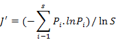
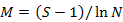
To enable comparisons between densities at replicates, the number of individuals and masses were standardised to 1000 m2 trawled area hauls (Linse et al., 2013). For each sample, the species number (S), Simpson diversity index (D), Shannon-Wiener index (H′), Pielou evenness (J′), Margalef index (M) and total abundance were calculated to describe the diversity of this area, which we calculated based on the abundance value. All the formulas were listed in Table II.

For the difference in the environmental characteristic of each sampling station, cluster analysis in average method and multidimensional scaling ordination (MDS) analysis were used based on Euclidean distance with square-root transformed and normalized data. Permutation test of variance analysis was previously done to test the hypothesis that variables of sediment and water column among clusters, and when test was significant (P < 0.05), a Duncan test (P < 0.05) based on permutation test model of variance was done to identify significant differences between pairs of clusters. When this was not possible, a Fisher-LSD test (P < 0.05) based on permutation test model of variance was done. A distance-based multivariate analysis of variance (PERMANOVA; Veiga et al., 2017) was used to test differences among clusters on the multivariate structure of environmental characteristic based on Euclidean distances by permutation of residuals under a reduced model (999 permutations). For each replicate, values of environmental variations were square-root transformed and normalized to reduce the influence of outliers.

Spatial variation in the macrobenthic community structure was evaluated using Fuzzy c-means clustering analysis (FCCA) and principal coordinates ordination (PcoA) analysis (Bezdek, 2011; Yan et al., 2017).

 

Table II.- Formulas for macrobenthos diversity calculations.

Biodiversity index	Connotation	Formulas	Remark
Simpson diversity index (D)	Dominance of familiar species		Pi means the ratio of Ni with the individual numbers of all the species; Ni means the individual numbers of the i species; S means the number of species
Shannon-Wiener index (H′)	Richness and evenness
Pielou evenness (J′)	Evenness
Margalef index (M)	Richness

 

Bray-Curtis similarity matrices based on fourth root transformed abundance datawrer constructed before the analysis (Yan et al., 2017). A PERMANOVA hypothesis test (999 permutations), as the aforementioned above, was applied to assess differences among groups on the multivariate structure of macrobenthic assemblages. Similarity percentage procedure (SIMPER) analysis was used to identity the species that contributed the most to the Bray-Curtis dissimilarity between the macrobenthic assemblages at each group (Clarke, 1993). A taxon was considered important if its contribution (δi) to total percentage dissimilarity was ≥ 3%. The ratio δi/SD (δi) was calculated to quantify the consistency in all pair-wise comparisons of groups. Values ≥ 1 indicated a high degree of consistency (Veiga et al., 2017).

 

The relationship between multivariate macrobenthic data and environmental variables of sedimentary environment and water column was analyzed using correspondence analysis based on fourth root transformed abundances and log(x+1) transformed environmental variables (Feld and Hering, 2010). Before that, conditional inference trees based on chi-square-type test statistics using the identity influence function for multivariate responses of five diversity indexes and abundance with fourth root transformed and asymptotic χ2 distribution are applied to select the fitted-environmental variables. For the criterion, values of the test statistic (Testatatistic) were used and we follow the usual convention by choosing the nominal level of the conditional independence tests as α = 0.95 (Hothom et al., 2006). Then, we relied on detrened correspondence analysis (DCA) to decide which correspondence analysis method is more suitable. If the maximum length of the axes was > 4SD, then constrained correspondence analysis (CCA) was more suitable and if the maximum length of the axes was < 3SD, then redundancy correspondence analysis (RDA) was more suitable, when the maximum length of the axes was between 3SD and 4SD, each method can be done (Yan et al., 2017). CCA was done to explicitly investigate the relationship between environmental variables and macrobenthic assemblages, because in preliminary DCA, the maximum gradient length of the axes was 3.95SD, is more closer to 4SD. P values were done using 999 permutations for CCA, and the significance of fitted variables is assessed using permutation (999) (Anderson, 2001).

 

Table III.- Result of PERMANOVA testing differences in the cluster of environmental variables. Analysis based on euclidean distance from square-root transformed and normalized data. All test used 999 random permutations.

Source of variation	df	MS	Pseudo-F	Unique perms
Cluster	3	0.3396	44.76***	999
Residuals	26	0.0076
Total	29

*, P < 0.05; **, P < 0.01; ***, P < 0.001.

 

Results

Environmental variables

Cluster analysis and MDS ordination visualized the variation in the environmental variables structure among the localities. Environmental variables from 30 stations were classified in to four clusters at 0.2 Euclidean distance (Fig. 2). PERMANOVA analysis indicated that the multivariate structure of environmental variables differed significantly among clusters (Table III). Cluster 4 was the largest, consisting 12 stations. This was followed by Cluster 2 (11 stations), Cluster 3 (6 stations) and Cluster1 (1 station). The character in Cluster 1 is high ammonium (0.030 ± 0.001 mg·L-1, (mean ± standard deviation (SD))), nitrate (0.656 ± 0.006 mg·L-1), pH (8.10 ± 0.01), reactive phosphorus (0.042 ± 0.0003 mg·L-1) and suspended matter (652.5 ± 59.5 mg·L-1). Cluster 2 is characterized by high sedimentary sulfide ((19.8 ± 31.6) × 10-6), sedimentary total nitrogen ((483.3 ± 60.6) × 10-6), sedimentary total phosphorus ((384.1 ± 45.5) × 10-6), nitrite (0.115 ± 0.005 mg·L-1), temperature (29.3 ± 0.5 °C) and water transparency (0.59 ± 0.19 m). For Cluster 3, water colour (20 ± 1), dissolved oxygen (6.65 ± 0.17 mg·L-1), depth (11.0 ± 2.5 m) and salinity (27.65 ± 1.00) are the highest. Sedimentary organic carbon ((0.48 ± 0.05) ×10-6) and reactive silicate (1.24 ± 0.25 mg·L-1) in Cluster 4 are the highest (Fig. 3). Permutation test of variance analysis showed that sediment sulfide, sediment total phosphorus, depth, nitrite and dissolved oxygen were not significant different among clusters (P > 0.05) and for these variables we used Fisher-LSD test to compare pairs and other environmental variables were significant (P < 0.05) (Table IV), for these variables, a Duncan test was done. The result of Fisher-LSD test and Duncan test were showed in Figure 3.

 

Table IV.- Results of permutation test of variance analysis in environmental variables among clusters.

		Source of variation (MS)		F-value
		Cluster (df=3)	Residuals (df=86)
Sedimentary
	Sulfide	1043.7	682.8	1.53
	Organic carbon	0.023	0.006	3.65*
	Total nitrogen	10648	2551	4.17**
	Total phosphorus	3196	1201	2.66
Water colour		31.423	1.313	23.94***
Depth		12.008	6.127	1.96
pH		0.0030	0.0002	13.08***
Salinity		5.727	0.846	6.77***
Suspended matter		532.707×103	6.040×103	88.20***
Temperature		1.813	0.202	9.00***
Water transparency		0.707	0.022	31.62***
Dissolved oxygen		0.079	0.038	2.15
Nitrite		4.985×10-5	1.844×10-5	2.70
Nitrate		0.119	0.007	16.87***
Reactive phosphorus		60.12×10-5	3.48×10-5	17.27***
Reactive silicate		0.768	0.066	11.69***
Ammonium		3.223×10-4	0.702×10-4	4.59**

*, P < 0.05; **, P < 0.01; ***, P < 0.001.

 

Macrobenthic assemblages

In total, 7446 individuals, recorded from 150 AGT catches in the ECS of Xiangshan, which belongs to seven phylum (Annelida, Arthropoda, Chordata, Cnidaria, Ctenophora, Echinodermata and Mollusca) and 36 taxa were identified throughout the study. Two of the most frequently observed macrobenthic were Arthropoda (100.0% of the total of stations) and Chordata(76.7%). Arthropoda and Chordata accounted for > 75% of the total macrobenthic species in most stations (Fig. 4). The average abundance of macrobenthic in ECS of Xiangshan is 239 ind/1000m2 and the maximum abundance occurs at S08 station (833 ind/1000m2) (Fig. 5B). The relative numbers and abundances of Arthropoda were both the highest one in the most stations (Fig. 4A). The overall trend of relative number of species and relative abundance in each stations were basically the same (Fig. 4). The result of diversity indexes are showed in Figure 5.

FCCA and PcoA analysis showed that the macrobenthic community significantly changed over stations (Fig. 6). Three groups were spread at 0.19 total average silhouette width. Group1 was composed 17 stations, Group2 composed 6 stations and Group3 composed 7 stations (Fig. 6A). PcoA also showed similar results. The first two axes explained 41.8% of total variation (Fig. 6B).

 

PERMANOVA analysis indicated that the multivariate structure of macrobenthic assemblages differed significantly among groups (Table V). SIMPER analysis showed that all the taxa were responsible for differences between groups. Collectively, these taxa contributed more than 80% to the total dissimilarity, although only the contribution by 11 of them was ≥ 3%. Oratosquilla oratoria, Palaemon gravieri, Parapenaeopsis hardwickii, Pleurobrachia globosa and Solenocera crassicornis were consistent among all the pair-wise comparisons between Group1, Group2 and Group3. Alpheus japonicus and Collichthys lucidus were consistent among the pair-wise comparisons of Group1 with Group2 and Group3. Acaudina molpadioides, Cavernularia obesa and Siliqua minima were consistent among the pair-wise comparisons of Group3 with Group1 and Group2. Nassarius variciferus contributed only to dissimilarity of Group2 and Group3 (Table VI).

 

Table V.- Result of PERMANOVA testing differences in the structure of macrobenthic assemblage among groups. Analysis based on Bray-Curtis dissimilarity from fourth root transformed data. All test used 999 random permutations.

Source of variation	df	MS	Pseudo-F	Unique perms
Group	2	0.9789	6.29	999
Residuals	27	0.1557
Total	29

 

Table VI.- Contribution of individual taxa to the average Bray-Curtis dissimilarity among groups that showed significant difference in the structure of their assemblages.

Species	Average abundance			Group1-Group2		Group1-Group3		Group2-Group3
	Group1	Group2	Group3	δi (%)	δi/SD	δi (%)	δi/SD	δi (%)	δi/SD
Acaudina molpadioides	1.35	0.00	14.01	0.51	0.35	3.74	0.46	6.12	0.45
Acetes chinensis	3.45	4.08	0.83	1.45	0.91	0.89	0.64	1.81	0.84
Alpheus japonicus	48.96	5.35	0.00	8.49	0.99	8.10	0.95	2.48	0.67
Anadara kagoshimensis	14.48	0.00	0.00	2.27	0.27	2.11	0.27	—	—
Anthopleura asiatica	0.00	0.00	2.67	—	—	0.65	0.70	1.23	0.67
Anthopleura japonica	0.00	0.00	11.43	—	—	1.79	0.39	2.52	0.40
Anthopleura nigrescens	0.00	0.00	1.26	—	—	0.33	0.37	0.58	0.39
Cavernularia obesa	1.05	4.18	16.55	1.29	0.46	3.88	1.35	6.96	1.31
Chaeturichthys stigmatias	1.54	0.00	0.00	0.32	0.36	0.29	0.35	—	—
Charybdis japonica	5.85	0.00	0.87	1.17	0.62	1.16	0.67	0.73	0.37
Collichthys lucidus	17.29	0.00	3.00	3.11	0.62	3.07	0.69	0.85	0.61
Cultellus attenuatus	0.63	0.00	0.00	0.20	0.25	0.18	0.24	—	—
Cynoglossus semilaevis	9.05	0.00	1.67	2.37	0.86	2.01	0.85	1.03	0.55
Ennucula faba	0.97	0.00	0.00	0.25	0.30	0.22	0.30	—	—
Harpadon nehereus	5.51	0.00	5.13	1.50	0.69	1.65	0.98	1.81	1.06
Larimichthys polyactis	1.34	0.00	0.00	0.33	0.38	0.29	0.37	—	—
Leptochela (Leptochela) gracilis	6.25	2.18	0.00	2.15	0.52	1.87	0.47	1.07	0.85
Metridium sinensis	0.00	0.00	0.92	—	—	0.23	0.38	0.39	0.39
Mierspenaeopsis cultrirostri	3.94	0.00	0.00	1.05	0.31	0.95	0.31	—	—
Nassarius variciferus	2.98	0.00	11.48	0.96	0.53	2.39	0.68	3.02	0.60
Nibea albiflora	4.72	0.00	0.00	1.01	0.59	0.92	0.58	—	—
Odontamblyopus rubicundus	5.80	1.04	3.00	1.66	0.77	1.59	0.82	1.13	0.75
Oratosquilla oratoria	21.84	8.30	5.89	4.32	1.24	4.86	1.38	4.09	1.50
Palaemon annandalei	1.15	2.27	0.00	1.12	0.53	0.46	0.24	1.24	0.62
Palaemon carinicauda	12.11	0.55	4.15	2.71	1.15	2.34	1.07	1.73	0.83
Palaemon gravieri	51.26	2.03	13.86	8.84	0.74	8.45	0.78	7.55	0.76
Parapenaeopsis hardwickii	44.12	4.09	13.14	9.37	1.01	8.78	1.04	6.00	0.70
Parapenaeopsis tenella	9.20	0.58	1.04	2.59	0.86	2.32	0.83	0.49	0.59
Perinereis aibuhitensis	1.12	0.00	1.04	0.27	0.39	0.36	0.53	0.23	0.40
Pleurobrachia globosa	3.51	50.72	18.77	13.16	1.25	4.00	0.96	18.51	1.17
Portunus (Portunus) sanguinolentus	0.00	0.00	0.80	—	—	0.29	0.35	0.66	0.37
Portunus (Portunus) trituberculatus	1.49	0.55	1.26	0.45	0.61	0.54	0.57	0.83	0.55
Protankyra bidentata	1.47	0.00	2.08	0.22	0.44	0.49	0.56	0.46	0.40
Raphidopus ciliatus	7.69	1.32	0.00	2.13	0.75	1.90	0.65	0.89	0.54
Siliqua minima	6.32	0.00	8.41	1.93	0.43	3.17	0.58	3.38	0.43
Solenocera crassicornis	31.98	6.91	4.44	7.52	1.09	6.77	1.05	3.74	0.91

Contributions were ≥ 3% indicated in bold.

 

Relationship between environmental variables and macrobenthic assemblages

The condition inference tree for specie abundances and diversity indexes (H′, D, J′, M) had one root node, six inner nodes and eight terminal nodes (Fig. 7). Six environmental variables (sedimentary sulfide, sedimentary organic carbon, sediment total phosphorus, water colour, dissolved oxygen and reactive phosphorus), associated with the response variables, were selected significantly. From the entire samples of 30 stations (represented by node one, where the node numbers are mere labels assigned recursively from left to right starting from the root node), a group of 14 stations is separated from the rest in the first split at the 3.6×10-6 level of the sedimentary sulfide, then further split into three groups (node3, node5, node6) by the water colour (18) and reactive phosphorus (0.038). The remaining 16 stations are further split into five groups (node8, node10, node13, node14 and node15) by the sedimentary organic carbon (0.44), sedimentary total phosphorus (348.5) and dissolved oxygen (6.56 and 6.49). The maximum value of H′, D, J′ and S were divided into node15, the character of this group is high sedimentary sulfide (>3.6), high sedimentary organic carbon (>0.44), high sedimentary total phosphorus (>348.5) and high dissolved oxygen (>6.56). The maximum value of M was divided into node3, this group means low sedimentary sulfide (<3.6) and low water colour. The maximum value of abundance is belong to node10, the character of this group is high sedimentary sulfide (>3.6), high sedimentary organic carbon (>0.44) but low sedimentary total phosphorus (<348.5) (Fig. 7).

 

Table VII.- Result of permutation test for constrained correspondence analysis. Number of permutations: 999.

Source of variation	df	Chi-Square	Pseudo-F	Unique perms
Group	6	0.612	1.28*	999
Residuals	23	1.835
Total	29

*, P < 0.05; **, P < 0.01; ***, P < 0.001.

 

The relationship between environmental variables and macrobenthic assemblages are illustrated in the CCA ordination diagram (Fig. 8). Permutation test indicated a high significant for the first two and all canonical axes (P < 0.05) (Table VII). The first two CCA axes explained 51.5% of the total variation of the species-environment relationship and 12.9% of the species variance. The goodness of fit statistic identified sedimentary sulfide (R2 = 0.4578, P < 0.001), sedimentary total phosphorus (R2 = 0.2013, P < 0.05), water colour (R2 = 0.3058, P < 0.05), dissolved oxygen (R2 = 0.4853, P < 0.001) as the important in relation to macrobenthic assemblages (Table VIII). The first CCA axes positively correlation with sedimentary sulfide (biplot scores is 0.3788), Sedimentary total phosphorus (0.9761), and negatively correlated with sedimentary organic carbon (-0.7561), water colour (0.1849). The second CCA axes positively correlation with sedimentary total phosphorus (0.2173), dissolved oxygen (0.6060), and negatively correlated with sedimentary sulfide (-0.9225) (Table VIII). The result of CCA analysis showed a clear distribution pattern of the stations and species with the fitted-environment variables (sedimentary sulfide, sedimentary total phosphorus, water colour and dissolved oxygen). The most of station in Group1 were positively correlation with the dissolved oxygen, water colour and sedimentary total phosphorus. The group2 was positively correlation with dissolved oxygen and water colour. Group3 was positively correlation with dissolved oxygen, sedimentary total phosphorus and sedimentary sulfide. The species were more positively correlation with dissolved oxygen, water colour and sedimentary sulfide (Fig. 8).

 

Table VIII.- The result of choice in displaying environmental variables in CCA analysis. Number of permutations: 999.

Environmental variables	CCA1	CCA2	R2
Sedimentary sulfide	0.3788	-0.9255	0.4578***
Sedimentary organic carbon	-0.7561	-0.6544	0.0887
Sedimentary total phosphorus	0.9761	0.2173	0.2013*
Water colour	-0.1849	0.9828	0.3058*
Dissolved oxygen	-0.7954	0.6060	0.4853***
Reactive phosphorus	0.2384	0.9712	0.1909

*, P < 0.05; **, P < 0.01; ***, P < 0.001.

 

Discussion

Environment spatial heterogeneity has a significantly impact on the distribution of macrobenthic assemblages (Meadows et al., 1998; Beisel et al., 2000). Cluster analysis for environmental variables in localities showed that the environmental variables had clear spatial heterogeneity in the ECS of Xiangshan. The four clusters had distinct dividing-line in space and present interlaced forms. Jiangsu Coastal Current (JCC), with relatively low temperature from circumpolar latitude, had less influence on water quality in the ECS of Xiangshan, as the Zhoushan Islands had formed a natural barrier to block JCC. Meanwhile, the density front between JCC and TWC spread the sea water to the offshore. This process complicated the situation of water disturbance in the study area. Cluster1 and cluster3, closed to the shore, were greatly affected by land-based sources pollution (Li and Daler, 2004) that produced by anthropogenic activities. Cluster1, cluster2 and cluster3, located in the entrance of Xiangshan Bay, which was an important aquafarm and sea-route (Li et al., 2012), were subjected to greater environmental pressure. These may be the reasons for the formation of environment spatial heterogeneity in the ECS of Xiangshan.

The spatial pattern of macrobenthic assemblages also had spatial heterogeneity. Fuzzy analysis and PcoA ordination showed that the macrobenthic assemblages significantly changed over spatial, but different from environmental spatial distribution. This means the variations in spatial patterns of macrobenthic assemblages were not fully explained by the studied variables of sediment and water column, and there were other abiotic or biotic variables were not considered in our study, such as sediment characteristics, median size, food supply, source of larvae or interspecies competition might also play a significant role (Wildish, 1977; Iván et al., 2009; Qunhau et al., 2017; Hua et al., 2017). Arrighetti and Penchaszadeh (2010) suggested that sediment characteristics were a key role of the spatial patterns of macrobenthic assemblages. Iván et al. (2009) found that the food quality was a structuring factor in macrobenthic communities. Previous research showed that aquaculture contributed to the spatial patterns of macrobenthos assemblages (Edgar et al., 2005). The adaptability of biological matter is one of its most striking and important properties (Conrad, 1976), defined as an ability to cope with abrupt environmental changes (Conrad and Calow, 1986). However, the opportunity bearing potential ability to colonize in stressed environments are divergent (Amri et al., 2014a). The proportion of species appeared in only some particular stations, such as Acaudina molpadioides and Perinereis aibuhitensis, they are more suitable for the soft sediment environment. In addition, the competition, predation, parasitism and symbiotic relationships between macrobenthos may also affect the spatial patterns of macrobenthic assemblages.

Identifying major environmental variables that shape distribution of macrobenthic assemblages is not an easy task, as they always change among space and different interacting factors may be involved (Lu, 2005). The relationship between the spatial patterns of macrobenthic assemblages and the environmental variables was directly related to the selected type of data in local condition (Xie et al., 2016). Veiga et al. (2017) used non-parametric multivariate regressions to exclude the redundant variables. Nishijima et al. (2015) taken principle component analysis (PCA) to decide the most important environmental variables. However, all of these methods are based on univariate analysis. Xie et al. (2016) suggested that the biological parameters reflecting different aspects of the macrobenthic structure should be taken into consideration when studying the relationships between macrobenthic structure and environmental variables. In present study, we used conditional inference trees based on chi-square-type test statistics using the identity influence function for multivariate responses of five diversity indexes and abundance to decide the fitted-environmental variables. Result indicated that sedimentary sulfide, sedimentary organic carbon, sediment total phosphorus, water colour, dissolved oxygen and reactive phosphorus were significantly associate with the response variables (macrobenthic diversity indexes and abundance).

The result of CCA highlighted that the spatial patterns of macrobenthic assemblages significantly correlated with sedimentary sulfide, sedimentary total phosphorus, dissolved oxygen and water colour. The variation of dissolved oxygen at the depth gradient was significant, conventionally the concentration of dissolved oxygen at the bottom was lower than that of surface layer due to the upper water column was more susceptible to wind disturbance (Dauer et al., 1992). And in marine sediments, anaerobic metabolism is generally the most important pathway for organic matter oxidation, among this processes, sulfate reduction usually plays the predominant role (Liu et al., 2014), resulting in the release of dissolved sulfides (Kanaya et al., 2015). Dissolved sulfides such as H2S is highly toxic to most macrobenthos, because it inhibits aerobic respiration (Bent, 1991). Dissolved oxygen content was an important natural environmental variable affecting the abundance and spatial patterns of macrobenthic assemblages (Verneaux et al., 2004). The concentration of sedimentary sulfide is opposite to the concentration of dissolved oxygen, as the anaerobic metabolism would be suppressed. As was showed in our research, cluster1 and cluster3 had lower concentrations of sedimentary sulfide, but their dissolved oxygen was higher, the opposite happened in cluster2 and cluster4. Meanwhile, diversity indexes of cluster1 and cluster3 were also higher. Phosphorus is one of the major elemental for life that plays a key role in marine primary productivity, which influences the global biogeochemical cycles (Elser et al., 2007; Defforey and Paytan, 2017). Primary producers are the main source of macrobenthos, and the increase of primary producers contributes to the increase in the biomass of macrobenthos (Amri et al., 2014b). Food availability is a key for macrobenthic assemblages (Dobson and Hildrew, 1992; Beisel et al., 2000). But too much phosphorus is beneficial to eutrophication (Conley et al., 2009), which has negative effects on macrobenthos assenblages: changes in species composition and changes in the behavior of species sensitive to reduced (Rodilla et al., 2006). Variation of marine surface optical properties are due to dissolved and suspended materials, with different absorption and scattering characteristics, present in sea water. In open sea waters, the pigments due to biological activities, and particularly phytoplankton chlorophyll-like pigments, are the main contributors to surface colour (Barale, 1991). It means the water colour, to a certain extent, represents the size of the biomass of primary producers, which indirectly affecting the spatial patterns of macrobenthic assemblages. Such as cluster2, with low abundance and low diversities, and its water colour is also low.

 

Conclusions

Field investigations were carried out at 30 stations in the ECS of Xiangshan. In total, 7446 individuals, which belong to seven phylum and 36 taxa were identified throughout the study. The environment of the study area has significant spatial heterogeneity caused by geographically, hydrodynamic and anthropogenic activities. Biotic variables should be considered in the research of macrobenthic distribution. When studying the relationships between spatial attempts of macrobenthic assemblages and environmental variables biological parameters need to be involved in many aspects. Sedimentary sulfide, sedimentary total phosphorus, dissolved oxygen and water colour are the certain environmetal factors that have proved shaping the distribution of macrobenthic abundance, diversity and multivariate structure of the assemblages.

 

Acknowledgments

This work was financially supported by National Special Research Fund for Non-Profit (No. 20130304), the Ningbo Marine Fisheries Service (No. E01207135300 and 81120314), and the K.C. Wong Magan Fund in Ningbo University. We thank Ningbo Academy of Oceanology and Fishery for providing sampling tools. We would also like to thank laboratory ember for supports and guidance throughout this study.

 

Statement of conflict of interest

Authors have declared no conflict of interest.

 

References

Amri, N., Jamili, S. and Abdolbaghian, S., 2014a. Diversity of macrobenthos communities and their relationships with environmental factors in Jajroud River, Iran. Resour. Environ., 4: 95-103.

Amri, N., Jamili, S. and Shahidian, M., 2014b. A study on the primary production of periphyton epilithics and biomass macrobenthos in Kordan River (North West of Iran). Int. J. Ecosyst., 4: 75-82.

Anderson, D.M., Glibert, P.M., Burkholder, J.M., Rabalais, N.N. and Nixon, S.W., 2002. Harmful algal blooms and eutrophication: Nutrient sources, composition, and consequences. Estuar. Coast., 25: 704-726. https://doi.org/10.1007/BF02804901

Anderson, M.J., 2001. Permutation tests for univariate or multivariate analysis of variance and regression. Can. J. Fish. aquat. Sci., 58: 626-639. https://doi.org/10.1139/f01-004

Arrighetti, F. and Penchaszadeh, P.E., 2010. Macrobenthos-sediment relationships in a sandy bottom community off Mar Del Plata, Argentina. J. Mar. Biol. Assoc. UK., 90: 933-939. https://doi.org/10.1017/S0025315409991524

Banse, K., Falls, C.P. and Hobson, L.A., 1963. A gravimetric method for determining suspended matter in sea water using millipore filters. Deep-Sea Res. Oceanogr. Abstract, 10: 639-642. https://doi.org/10.1016/0011-7471(63)90005-6

Barale, V., 1991. Sea surface colour in the field of biological oceanography. Int. J. Remote Sens., 12: 781-793. https://doi.org/10.1080/01431169108929694

Beisel, J.N., Philippe, U.P. and Moreteau, J.C., 2000. The spatial heterogeneity of a river bottom: a key factor determining macroinvertebrate communities. Hydrobiologia, 422-423: 163-171. https://doi.org/10.1023/A:1017094606335

Bent, V., 1991. Sulfide tolerance: Physiological mechanisms and ecological implications. Ophelia, 34: 1-27. https://doi.org/10.1080/00785326.1991.10429703

Bezdek, J., 2011. Fuzzy C-means cluster analysis. Scholarpedia, 6: 2057. https://doi.org/10.4249/scholarpedia.2057

Blanchet, H., Montaudouin, X.D., Chardy, P. and Bachelet, G., 2005. Structuring factors and recent changes in subtidal macrozoobenthic communities of a coastal lagoon, Arcachon Bay (France). Estuar. Coast. Shelf. Sci., 64: 561-576. https://doi.org/10.1016/j.ecss.2005.03.016

Chen, C.C., Gong, G.C. and Shiah, F.K., 2007. Hypoxia in the East China Sea: One of the largest coastal low-oxygen areas in the world. Mar. Environ. Res., 64: 399-408. https://doi.org/10.1016/j.marenvres.2007.01.007

Clarke, K.R., 1993. Nonparametric multivariate analysis of changes in community structure. Aust. J. Ecol., 18: 117-143. https://doi.org/10.1111/j.1442-9993.1993.tb00438.x

Claudet, J. and Fraschetti, S., 2010. Human-driven impacts on marine habitats: A regional meta-analysis in the Mediterranean Sea. Biol. Conserv., 143: 2195-2206. https://doi.org/10.1016/j.biocon.2010.06.004

Conley, D.J., Paerl, H.W., Howarth, R.W., Boesch, D.F., Seitzinger, S.P., Havens, K.E., Christiane, L. and Likens, G.E., 2009. Controlling eutrophication: Nitrogen and phosphorus. Science, 323: 1014. https://doi.org/10.1126/science.1167755

Conrad, M., 1976. Biological adaptability: The statistical state model. BioScience, 26: 319-324. https://doi.org/10.2307/1297372

Conrad, M. and Calow, P., 1986. Adaptability: The significance of variability from molecule to ecosystem. Bull. Math. Biol., 48: 701-703. https://doi.org/10.1007/BF02462331

Crawford, C.M., Macleod, C.K.A. and Mitchell, I.M., 2003. Effects of shellfish farming on the benthic environment. Aquaculture, 224: 117-140. https://doi.org/10.1016/S0044-8486(03)00210-2

Dauer, D.M., Rodi, A.J. and Ranasinghe, J.A., 1992. Effects of low dissolved oxygen events on the macrobenthos of the lower Chesapeake Bay. Estuar, Coast., 15: 384-391. https://doi.org/10.2307/1352785

Dauvin, J.C., 2007. Paradox of estuarine quality: Benthic indicators and indices, consensus or debate for the future. Mar. Pollut. Bull., 55: 271-281. https://doi.org/10.1016/j.marpolbul.2006.08.017

Defforey, D. and Paytan, A., 2017. Phosphorus cycling in marine sediments: Advances and challenges. Chem. Geol., 477: 1-11. https://doi.org/10.1016/j.chemgeo.2017.12.002

Desroy, N., Warembourg, C., Dewarumez, J.M. and Dauvin, J.C., 2003. Macrobenthic resources of the shallow soft-bottom sediments in the eastern English Channel and southern North Sea. ICES J. Mar. Sci., 60: 120-131. https://doi.org/10.1006/jmsc.2002.1333

Dobson, M. and Hildrew, A.G., 1992. A test of resource limitation among shredding detritivores in low order streams in Southern England. J. Anim. Ecol., 61: 69-77. https://doi.org/10.2307/5510

Dolbeth, M., Ferreira, Ó., Teixeira, H., Marques, J.C., Dias, J.A. and Pardal, M.A., 2007. Beach morphodynamic impact on a macrobenthic community along a subtidal depth gradient. Mar. Ecol. Prog. Ser., 352: 113-124. https://doi.org/10.3354/meps07040

Edgar, G.J., Macleod, C.K., Mawbey, R.B. and Shields, D., 2005. Broad-scale effects of marine salmonid aquaculture on macrobenthos and the sediment environment in southeastern Tasmania. J. exp. Mar. Biol. Ecol., 327: 70-90. https://doi.org/10.1016/j.jembe.2005.06.003

Edwards, A.H., 2007. The semi-micro Kjeldahl method for the determination of nitrogen in coal. J. appl. Chem., 4: 330-340.

Elser, J.J., Bracken, M.E., Cleland, E.E., Gruner, D.S., Harpole, W.S., Hillebrand, H., Jacqueline, T.N., Eric, W.S., Jonathan, B.S. and Jennifer, E.S., 2007. Global analysis of nitrogen and phosphorus limitation of primary producers in freshwater, marine and terrestrial ecosystems. Ecol. Lett., 10: 1135-1142. https://doi.org/10.1111/j.1461-0248.2007.01113.x

Feld, C.K. and Hering, D., 2010. Community structure or function: effects of environmental stress on benthic macroinvertebrates at different spatial scales. Freshw. Biol., 52: 1380-1399. https://doi.org/10.1111/j.1365-2427.2007.01749.x

Gong, G.C., Chang, J., Chiang, K.P., Hsiung, T.M., Hung, C.C., Duan, S.W. and Codispoti, A., 2006. Reduction of primary production and changing of nutrient ratio in the east china sea: effect of the three gorges dam? Geophys. Res. Lett., 33: 3716-3730. https://doi.org/10.1029/2006GL025800

Hothorn, T., Hornik, K. and Zeileis, A., 2006. Unbiased recursive partitioning: a conditional inference framework. J. Comput. Graph., 15: 651-674. https://doi.org/10.1198/106186006X133933

Hua, L.S., Gong, S., Zhong, X.J., Tao, J., Chen, Y. and Deng, J.M., 2017. The effects of water depth and substrate conditions on changes in body weight and health status of captive big-headed turtles (Platysternon megacephalum) during hibernation. Pakistan J. Zool., 49: 2243-2248. https://doi.org/10.17582/journal.pjz/2017.49.6.2243.2248

Iván, F.R., Mariano, L. and Jesús, L., 2009. Spatial variability of benthic macrofauna in the Ria of Vigo (NW Spain): Effect of sediment type and food availability. Mar. Biol. Res., 5: 572-584. https://doi.org/10.1080/17451000902729688

Ivanov, K., Zaprjanova, P. and Petkova, M., 2012. Comparison of inductively coupled plasma mass spectrometry and colorimetric determination of total and extractable phosphorus in soils. Spectrochim. Acta Part B: Atom. Spectrosc., 71-72: 117-122. https://doi.org/10.1016/j.sab.2012.05.013

Jiang, Z., Liu, J., Chen, J., Chen, Q., Yan, X., Xuan, J. and Zeng, J., 2014. Responses of summer phytoplankton community to drastic environmental changes in the Changjiang (Yangtze River) estuary during the past 50 years. Water Res., 54: 1-11. https://doi.org/10.1016/j.watres.2014.01.032

Kanaya, G. and Kikuchi, E., 2004. Relationships between sediment chemical buffering capacity and H2S accumulation: comparative study in two temperate estuarine brackish lagoons. Hydrobiologia, 528: 187-199. https://doi.org/10.1007/s10750-004-2342-8

Kanaya, G., Nakamura, Y., Koizumi, T. and Yamada, K., 2015. Seasonal changes in infaunal community structure in a hypertrophic brackish canal: Effects of hypoxia, sulfide, and predator-prey interaction. Mar. Environ. Res., 108: 14-23. https://doi.org/10.1016/j.marenvres.2015.04.006

Keeley, N.B., Macleod, C.K., Hopkins, G.A. and Forrest, B.M., 2014. Spatial and temporal dynamics in macrobenthos during recovery from salmon farm induced organic enrichment: when is recovery complete? Mar. Pollut. Bull., 80: 250-262. https://doi.org/10.1016/j.marpolbul.2013.12.008

Konda, M., Imasato, N. and Shibata, A., 2002. Interannual variability of the sea-surface temperature in the Indian Ocean in response to the air-sea turbulent heat exchange. Deep-Sea Res. Part II, 49: 1527-1548. https://doi.org/10.1016/S0967-0645(01)00162-X

Kumar, K., Anneboina, L.R., Bhatta, R., Naren, P., Nath, M., Sharan, A., Mukhopadhyay, P., Ghosh, S., Costa, V. and Pednekar, S., 2016. Valuation of coastal and marine ecosystem services in India: Macro assessment. Monograph No. 35/2016. Madras School of Economics, Chennai, India.

Large, S.I., Fay, G., Friedland, K.D. and Link, J.S. 2015. Quantifying patterns of change in marine ecosystem response to multiple pressures. PLoS One, 10: e0119922. https://doi.org/10.1371/journal.pone.0119922

Lee, H.J. and Chao, S.Y., 2003. A climatological description of circulation in and around the east china sea. Deep-Sea Res. Part II, 50: 1065-1084. https://doi.org/10.1016/S0967-0645(03)00010-9

Li, D. and Daler, D., 2004. Ocean pollution from land-based sources: East China Sea, China. AMBIO A J. Hum. Environ., 33: 107. https://doi.org/10.1579/0044-7447-33.1.107

Li, M., Xu, K., Watanabe, M. and Chen, Z., 2007. Long-term variations in dissolved silicate, nitrogen, and phosphorus flux from the Yangtze River into the East China Sea and impacts on estuarine ecosystem. Estuar. Coast. Shelf. Sci., 71: 3-12. https://doi.org/10.1016/j.ecss.2006.08.013

Li, W., Yang, H., Gao, Q., Pan, H. and Yang, H., 2012. Residues of organochlorine pesticides in water and suspended particulate matter from Xiangshan Bay, East China Sea. Bull. Environ. Contam. Toxicol., 89: 811-815. https://doi.org/10.1007/s00128-012-0777-6

Linse, K., Griffiths, H.J., Barnes, D.K., Brandt, A., Davey, N., David, B., Grave, A.D., d’Acoz, C.D., Eléaume, M., Adrian G.G., Lenaïg, G.H., Christopher, M., Rafael, M.L., Tomás, M., Mark, O.L., Pierrat, B., Saucède, T., Chester, J.S., Strugenll, J.M. and Enderlein, P., 2013. The macro- and megabenthic fauna on the continental shelf of the eastern Amundsen Sea, Antarctica. Cont. Shelf. Res., 68: 80-90. https://doi.org/10.1016/j.csr.2013.08.012

Liu, J., Zhu, M. X., Yang, G.P., Shi, X. N. and Yang, R.J., 2014. Quick sulfide buffering in inner shelf sediments of the East China Sea impacted by eutrophication. Environ. Earth Sci., 71: 465-473. https://doi.org/10.1007/s12665-013-2454-4

Liu, J.P., Li, A.C., Xu, K.H., Velozzi, D.M., Yang, Z.S., Milliman, J.D. and DeMaster, D.J., 2006. Sedimentary features of the Yangtze River-derived along-shelf clinoform deposit in the East China Sea. Cont. Shelf. Res., 26: 2141-2156. https://doi.org/10.1016/j.csr.2006.07.013

Lu, L., 2005. The relationship between soft-bottom macrobenthic communities and environmental variables in Singaporean waters. Mar. Pollut. Bull., 51: 1034-1040. https://doi.org/10.1016/j.marpolbul.2005.02.013

Lu, S., Liao, Y., Tang, Y., Chen, J., Jiang, Z., Gao, A. and Chen, Q., 2017. Seasonal distribution of macrobenthos and its relationship with environmental factors in Yellow Sea and East China Sea. Chin. J. Oceanol. Limnol., 35: 1-11. https://doi.org/10.1080/14634988.2013.759497

Lu, S., Zeng, J., Liao, Y., Xu, T., Gao, A., Chen, Z., Chen, Q. and Yang, J., 2013. Temporal and spatial variability of benthic macrofauna communities in the Yangtze River estuary and adjacent area. Aquat. Ecosys. Hlth., 16: 31-39.

McGlade, C. and Ekins, P., 2015. The geographical distribution of fossil fuels unused when limiting global warming to 2°C. Nature, 517: 187. https://doi.org/10.1038/nature14016

Meadows, A., Meadows, P.S. and Mclaughlin, P., 1998. Spatial heterogeneity in an intertidal sedimentary environment and its macrobenthic community. Geol. Soc. London Spec. Publ., 139: 367-388. https://doi.org/10.1144/GSL.SP.1998.139.01.28

Munari, C. and Mistri, M., 2008. The performance of benthic indicators of ecological change in adriatic coastal lagoons: throwing the baby with the water? Mar. Pollut. Bull., 56: 95-105. https://doi.org/10.1016/j.marpolbul.2007.09.037

Nishijima, W., Umehara, A., Okuda, T. and Nakai, S., 2015. Variations in macrobenthic community structures in relation to environmental variables in the Seto Inland Sea, Japan. Mar. Pollut. Bull., 92: 90. https://doi.org/10.1016/j.marpolbul.2014.12.051

Pawlowski, L., 1994. Standard methods for examination of water and waste water, 18th edition. Sci. Total Environ., 142: 227-228.

Pratt, D.R., Lohrer, A.M., Pilditch, C.A. and Thrush, S.F., 2014. Changes in ecosystem function across sedimentary gradients in estuaries. Ecosystems, 17: 182-194. https://doi.org/10.1007/s10021-013-9716-6

Qunhau, H., Meiwen, Z., Cong, G., Xunjun, Z., Bo, L. and Yong, W., 2017. Density effect on postnatal growth of laboratory-bred Yangtze Vole (Microtus fortis calamorum). Pakistan J. Zool., 49: 1953-1962. https://doi.org/10.17582/journal.pjz/2017.49.6.1953.1962

Rodilla, M., Martí, E., Falco, S., Río, J.G.D., Sierra, J.P. and Arcilla, A.S., 2006. Eutrophication of sediments in the Cullera Bay: Composition and abundance of macrobenthos. J. Coast. Res., 39: 1533-1537.

Schückel, U., Beck, M. and Kröncke, I., 2015. Macrofauna communities of tidal channels in jade bay (German Wadden Sea): Spatial patterns, relationships with environmental characteristics, and comparative aspects. Mar. Biodiv., 45: 1-15. https://doi.org/10.1007/s12526-014-0308-2

Sousa, R., Dias, S. and Antunes, J.C., 2006. Spatial subtidal macrobenthic distribution in relation to abiotic conditions in the Lima Estuary, NW of Portugal. Hydrobiologia, 559: 135-148. https://doi.org/10.1007/s10750-005-1371-2

Sparks, D.L., Page, A.L., Helmke, P.A., Loeppert, R.H., Nelson, D.W. and Sommers, L.E., 1996. Total carbon, organic carbon, and organic matter. Methods Soil Analy., 9: 961-1010.

Stohlgren, T.J. and Schnase, J.L., 2006. Risk Analysis for biological hazards: What we need to know about invasive species? Risk Analy., 26: 163-173. https://doi.org/10.1111/j.1539-6924.2006.00707.x

Tong, C., Baustian, J.J., Graham, S.A. and Mendelssohn, I.A., 2013. Salt marsh restoration with sediment-slurry application: Effects on benthic macroinvertebrates and associated soil-plant variables. Ecol. Eng., 51: 151-160. https://doi.org/10.1016/j.ecoleng.2012.12.010

Veiga, P., Redondo, W., Sousapinto, I. and Rubal, M., 2017. Relationship between structure of macrobenthic assemblages and environmental variables in shallow sublittoral soft bottoms. Mar. Environ. Res., 129: 369-407. https://doi.org/10.1016/j.marenvres.2017.07.002

Verneaux, V., Verneaux, J., Schmitt, A. and Lambert, J.C., 2004. Relationships of macrobenthos with dissolved oxygen and organic matter at the sediment-water interface in ten French lakes. Arch. Hydrobiol., 160: 247-259. https://doi.org/10.1127/0003-9136/2004/0160-0247

Wildish, D.J., 1977. Factors controlling marine and estuarine sublittoral macrofauna. Helgoland. Wiss. Meer, 30: 445-454. https://doi.org/10.1007/BF02207853

Xie, Z., Zhang, J., Cai, K., Xu, Z., Wu, D. and Wang, B., 2016. Temporal and spatial distribution of macrobenthos communities and their responses to environmental factors in Lake Taihu. Acta Ecol. Sin., 36: 16-22. https://doi.org/10.1016/j.chnaes.2015.12.005

Xu, Y., Li, X., Wang, H. and Zhang, B., 2016a. Seasonal and spatial variations of macrobenthic community structure and diversity in the South Yellow Sea. Aquat. Ecosyst. Hlth., 19: 92-100. https://doi.org/10.1080/14634988.2016.1139429

Xu, Y., Sui, J., Yang, M., Sun, Y., Li, X., Wang, H. and Zhang, B., 2016b. Variation in the macrofaunal community over large temporal and spatial scales in the southern Yellow Sea. J. Mar. Syst., 173: 9-20. https://doi.org/10.1016/j.jmarsys.2016.11.006

Yan, J., Xu, Y., Sui, J., Li, X., Wang, H. and Zhang, B., 2017. Long-term variation of the macrobenthic community and its relationship with environmental factors in the Yangtze River estuary and its adjacent area. Mar. Pollut. Bull., 123: 339-348. https://doi.org/10.1016/j.marpolbul.2017.09.023

Zhang, J.L., Xiao, N., Zhang, S., Xu, F. and Zhang, S., 2016. A comparative study on the macrobenthic community over a half century in the Yellow Sea, China. J. Oceanogr., 72: 189-205. https://doi.org/10.1007/s10872-015-0319-z